


| Issue |
EPJ Photovolt.
Volume 17, 2026
Special Issue on ‘EU PVSEC 2025: State of the Art and Developments in Photovoltaics', edited by Robert Kenny and Carlos del Cañizo
|
|
|---|---|---|
| Article Number | 22 | |
| Number of page(s) | 10 | |
| DOI | https://doi.org/10.1051/epjpv/2026014 | |
| Published online | 11 June 2026 | |
https://doi.org/10.1051/epjpv/2026014
Original Article
Simulation-based insights into light soaking and light-induced degradation in perovskite solar cells
1
Institut Photovoltaïque d’Île-de-France (IPVF), Palaiseau, 91120, France
2
Institut Photovoltaïque d'Île-de-France (IPVF), UMR 9006, CNRS, École Polytechnique, IP Paris, Chimie Paristech, PSL, Palaiseau, 91120, France
3
School of Photovoltaic and Renewable Energy Engineering, University of New South Wales, Sydney, NSW 2052, Australia
4
EDF R&D, Palaiseau, 91120, France
* e-mail: This email address is being protected from spambots. You need JavaScript enabled to view it.
Received:
16
December
2025
Accepted:
11
May
2026
Published online: 11 June 2026
Abstract
Perovskite solar cells have achieved remarkable power conversion efficiencies, yet their long-term stability remains a critical challenge. Progress in understanding this issue can be supported by combining modelling and characterization of the experimental behaviour obtained during ageing. Degradation studies often rely on post-mortem analysis, which is time-intensive, costly, and requires expertise. Here, we present a modelling framework that provides insights into the underlying mechanisms using simple electrical measurements performed during ageing tests. Drift-diffusion and transfer-matrix simulations of the cell optoelectronic response are combined with a genetic algorithm to reproduce the measured JV characteristics. By tracking the evolution of correlations between electrical parameters (VOC, JSC and FF), simulated mechanisms are compared with experimental data, enabling discrimination between feasible pathways associated with performance improvement during light soaking and light-induced degradation. These mechanisms are simulated by varying material parameters such as charge-carrier mobilities, doping levels, defect concentrations in the absorber and at the perovskite/transport-layer interfaces, and parasitic resistances. Comparison between experiment and simulation distinguishes mechanisms that are consistent with the measured trajectories from those that are not, while highlighting plausible candidates associated with both performance improvement during light soaking and light-induced degradation, thereby providing new insights into perovskite solar cell stability.
Key words: Perovskite solar cells / stability / degradation / light soaking / modelling / indoor ageing
© G. Álvarez Pérez et al., Published by EDP Sciences, 2026
 This is an Open Access article distributed under the terms of the Creative Commons Attribution License (https://creativecommons.org/licenses/by/4.0), which permits unrestricted use, distribution, and reproduction in any medium, provided the original work is properly cited.
1 Introduction
Renewable energy is set to play a vital role towards meeting the growing global energy demand and reducing emissions from the energy sector, which is responsible for nearly three-quarters of global greenhouse gas emissions [1]. Among renewable sources, solar photovoltaic technology is expected to be a key contributor to the energy transition.
Currently dominated by silicon-based technologies, the photovoltaic market is projected to grow substantially [2], highlighting the importance of developing efficient and cost-effective alternatives. Perovskite solar cells have attracted significant interest due to their impressive advancements in power conversion efficiency over the past decade, recently achieving single-junction devices with over 26% efficiency [3], but their stability remains an issue to be solved.
Several factors related to instabilities have been identified. Some of them are extrinsic to the devices, such as the presence of oxygen or humidity, and can be tackled by improving encapsulation and fabrication strategies. But some others, like the effect of temperature, illumination and voltage bias, are complex to solve [4,5]. Moreover, there is a lack of understanding of the physical parameters that lead to experimental instabilities. Thus, there is a need to have a better understanding of how these factors influence perovskite solar cells. This can help to provide insights into mitigating irreversible degradation and understanding light soaking effects.
While degradation of perovskite solar cells has already attracted the attention of the scientific community [4–6], studies frequently address degradation from a “post-mortem” perspective. Thus, there is still a limited understanding of the dynamic processes involved, as many different factors can make perovskite solar cells degrade. While research efforts have focused on mitigating degradation, performance improvement has received less attention, despite being widely reported. Since these phenomena are not necessarily independent, they should be studied together.
Experimental methods for studying instabilities are restricted due to high costs, time requirements, and reliance on expertise. This study combines modelling and characterization to investigate experimental instabilities in perovskite solar cells, offering insights into the mechanisms driving light-induced performance decline and light soaking responses. The analysis is conducted within a time-independent framework, eliminating the temporal dependence on activation factors or environmental conditions. Instead, the focus is on the evolutions of correlations of key electrical parameters: open-circuit voltage (VOC), short-circuit current (JSC), and fill factor (FF). The correlation evolution obtained experimentally serves as a footprint of the device's behaviour, showing the states the cells undergo along ageing. Comparing experimental and simulated correlation paths helps to discriminate the most and least probable mechanisms underlying these phenomena.
Related strategies have also been proposed to infer performance-limiting parameters from JV characteristics using data-driven methods trained on simulated device responses [7]. Whereas that work focuses on parameter inference from simulated JV datasets using machine learning, the present study analyses time-resolved ageing trajectories. It builds on the correlation-pathway concept introduced previously [8] and extends it to ageing of devices that captures both performance-increase and performance-loss phases within the same experiment.
The proposed approach enables the differentiation of mechanisms associated with performance-increase and performance-loss phases during ageing, based solely on time-resolved electrical measurements. By analysing how the device trajectory evolves in correlation space, the framework links laboratory observations to candidate underlying mechanisms, providing a structured way to interpret complex ageing dynamics. Importantly, discriminating mechanisms that act across multiple regimes from those linked mainly to performance loss can help target mitigation strategies and guide further experimental studies.
2 Methodology
Understanding instability mechanisms in perovskite solar cells is essential to mitigating losses. Coupling ageing data with modelling provides insights into the mechanisms behind experimental behaviour while avoiding further characterization, which is often expensive, time-consuming, expertise-dependent, added to the fact that it is not always straightforward to design mechanism-specific tests.
Different mechanisms are proposed to contribute to instabilities, guided by the existing literature on perovskite solar cell stability [4–8]. They are simulated by varying physical parameters associated with the layer properties, such as defect concentration in the absorber and interfaces, charge carrier mobilities, doping in transport layers and external series and shunt resistances. Mechanisms are computed individually, assuming they act independently. This assumption reduces the complexity of simulations and allows a direct comparison between simulated and experimental results, enabling the identification of which mechanisms have the largest impact on device performance.
2.1 Experimental data
For this study, eight perovskite solar cells were fabricated and characterized at IPVF. They were aged together for 1150 h, resulting in a total of 9200 h of ageing data. The devices originate from a preindustrial pilot-line fabrication workflow and were monitored within a reliability-oriented ageing campaign rather than optimized for record efficiency. Accordingly, the aim of this work is to demonstrate the proposed correlation-pathway methodology on long-term JV ageing datasets. Extension to higher-efficiency state-of-the-art devices will be addressed when comparable datasets become available. The absorber consists of a triple-cation perovskite, and the cells have the following nip structure: Glass/FTO/TiO2/ Cs0.05(MA0.17FA0.83)0.95Pb(Br0.17I0.83)3/PTAA/Au. The substrate area is 2 cm2 and the active area of the cells is 0.2 cm2.
The only differences between the cells are related to the perovskite precursor preparation: (i) timing of preparation: same day as spin-coating or one day in advance, and (ii) preheating at 70 °C for 1 h prior to deposition versus no preheating. Two devices were fabricated for each of the four resulting conditions. Devices are labelled as Cell 1.1–4.2 according to split group (see Tab. S1).
In terms of characterization, the solar cells were aged under maximum power point (MPP) tracking in a nitrogen atmosphere under constant AM1.5G illumination provided by an LED light source (100 mW/cm2), with the sample temperature monitored at approximately 32 °C. Device performance was monitored by periodic JV measurements every 15 min, first in forward and then in reverse scan, with a scan rate of 20 mV/s. Cells 1.1, 2.1 and 2.2 showed erratic behaviour and early failure and were excluded from the analysis.
Figure 1 presents the ageing results for the five devices analysed, showing the power conversion efficiency (PCE) evolution along time. It shows the temporal instabilities of perovskite solar cells. All of them experience a reduction in PCE related to performance loss, albeit at different rates. During the initial hours of testing, a light soaking period is observed, characterized by an increase in output power. This phase continues for approximately 60 to 70 h, after which all devices reach a maximum, followed by light-induced degradation.
The laboratory light source was switched off at 440 h, resulting in 12 h without direct illumination. Upon resuming illumination, a second light soaking period is observed, leading to a further increase in PCE over approximately 50 h. Figure 1 shows the trends for the first 600 h. The devices studied retained over 80% of their initial PCE after 1150 h, consistent with limited long-term degradation. For each device, both light soaking (LS) phases and the drop in performance in between them are considered to assess feasible mechanisms causing these phenomena. We refer to the performance decline under illumination as light-induced degradation (LID), and to the two performance increases after dark as first light soaking (LS1) and second light soaking (LS2). Here, the term light soaking is used to denote the post-dark illumination intervals in this ageing protocol during which the devices exhibit a net performance increase.
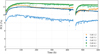 |
Fig. 1 Temporal evolution of the output power for the five solar cells studied under continuous illumination at 100 mW/cm2. Light soaking (LS1, LS2) and light-induced degradation (LID) phases are observed. LS1 starts at t = 0 h, LS2 at t = 452 h after light was interrupted for 12 h, and LID occurs between them. Device labels follow the notation defined in Table S1. |
2.2 Data processing
Raw data presented in Figure 1 is processed to select and extract trends of interest before running simulations. First, JV curves are smoothed along voltage for both forward and reverse scans. Next, the temporal variation of electrical parameters (VOC, JSC and FF) is computed and smoothed over time, and outliers are removed. Finally, the average of the forward and reverse JV curves is calculated to represent the overall cell’s behaviour and to reduce scan-direction differences. Such differences are often attributed to charge-displacement phenomena in perovskite solar cells (e.g., mobile ions and/or slow traps) [9–11], which are not explicitly included in the steady-state drift-diffusion framework used here. Ion/trap-aware drift-diffusion solvers would require introducing additional dynamic parameters (e.g., ionic densities/mobilities and characteristic time constants) which cannot be robustly constrained with the current JV data available and would substantially increase model dimensionality and computational cost. We therefore treat FW/RV averaging as an effective approximation. Further details on the data processing procedure are provided in the Supplementary material.
Simulations assume that a single material parameter dominates the evolution of each trend (performance increase or decline). Following this assumption, intervals are preferentially selected such that VOC, JSC and FF show an overall change in the same direction, as depicted in Figure 2. Intervals with clearly mixed trends are excluded for simplicity, since they may indicate multiple interacting mechanisms which are not trivial to disentangle from JV data alone. Among these, only segments showing an approximately linear evolution in PCE are retained, as these are expected to correspond more closely to a simpler ageing behaviour governed by one or a few dominant physical parameters.
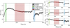 |
Fig. 2 Temporal evolution of the PCE, VOC, JSC, and FF for Cell 1.2 during the first 600 h. LID happens between LS1 and LS2, LS2 occurs at t = 452 h after light interruption. Notably, simultaneous performance increase and decline are selected across all parameters, reducing the complexity of feasible mechanisms behind instabilities and making the results interpretable. An identical selection and processing procedure was applied to all cells studied. |
2.3 Simulating ageing behaviour
Solar cells are modelled as one-dimensional structures constituted by three uniform layers with parallel interfaces: the perovskite absorber situated between the hole transport layer (HTL) and the electron transport layer (ETL). Different types of layers can be adapted based on material parameters of the cells studied, such as the thickness of the layers, their bandgap, and relative permittivity, among others (see material parameters listed in Tab. S2).
For each solar cell studied, its behaviour is simulated by combining optoelectronic and drift-diffusion models. Optical simulations, which model light propagation within the cell, are calculated by means of transfer matrix calculations. From the layers’ thicknesses and refractive indices, the generation rate is calculated. Subsequently, drift-diffusion simulations are performed with SCAPS [12], a one-dimensional numerical solver designed for thin-film solar cells, yielding the simulated JV characteristics that describe the electrical behaviour of the devices.
The starting point to simulate mechanisms is obtained by means of a genetic algorithm. It consists of sets of simulated devices that closely match the experimental data at the beginning of each trend studied. Each set has its own material parameters defined, from which performance increase/decline is computed.
2.3.1 Genetic algorithm
The genetic algorithm (GA) used in this study generates ensembles of drift-diffusion JV simulations that reproduce the experimental JV characteristics at the beginning of each interval studied [8]. Fitting drift-diffusion JV curves is a non-linear and generally non-unique inverse problem: multiple combinations of material parameters can reproduce very similar JV characteristics, often with parameters spanning orders of magnitude. For this reason, we do not aim to extract a single “best-fit” parameter set, but to generate an ensemble of near-optimal solutions that captures non-uniqueness and parameter correlations. A GA is well suited to explore this large, multi-dimensional parameter space and is less sensitive to the initial guess than local gradient-based optimizers, at the expense of higher (but reasonable) computational costs.
In practice, the GA starts by generating candidate parameter sets within physically motivated bounds (Tab. S2). These parameter sets are sampled using a log-uniform distribution, since many relevant material parameters naturally vary on logarithmic scales. Depending on the sample, an initial pool of 2000–4000 parameter sets is generated. For each candidate set, a JV curve is simulated and compared to experiment using a metric based on the relative error in VOC, JSC, and FF, as well as the slopes of the JV curves close to VOC and JSC. The candidates are then ranked, and only the best-performing subset is retained. In the proposed workflow, the 30 closest JV sets are selected and used to generate the next population.
The selected parameter sets are then mutated and re-evaluated, and this selection-mutation loop is repeated until convergence. Mutation is applied as a multiplicative rescaling on a logarithmic scale: each chosen parameter is multiplied by a random factor drawn continuously from a log-uniform range bounded by a maximum scaling factor. This allows variable-sized perturbations rather than fixed jumps. To balance exploration and convergence, the maximum scaling factor is set larger in the early iterations and progressively reduced, typically from about 2 at the beginning to about 1.25 close to the end of the GA. The iterations stop when the relative error between simulated and experimental electrical parameters falls below a tolerance, typically 3%.
The parameter space defined by Table S2 is extremely large (combinations on the order of 1010), so exhaustive exploration is neither feasible nor intended. The final output is an ensemble of approximately 100 parameter sets (and corresponding JV curves) that reproduce the experimental JV metrics within the prescribed tolerance. These retained parameter sets then serve as starting points for the simulations described in the following section.
2.3.2 Simulating performance increase and decline
Once the starting points are defined, the proposed mechanisms are simulated by varying material parameters one at a time. This procedure implicitly assumes that the mechanisms act independently during ageing. Although this is a simplifying assumption, introduced to limit the dimensionality of the problem and the associated computational cost, it already enables the identification of which mechanisms best reproduce the experimental behaviour.
The simulated mechanisms include variations in charge-carrier mobilities in the perovskite and transport layers, defect densities at the perovskite/transport-layer interfaces and in the perovskite bulk, doping levels in the transport layers, and the influence of external resistances.
For each of the 100 starting sets, the device response to a given parameter change is evaluated using the parameter ranges listed in Table S2, and the results are averaged over all 100 calculations. This ensemble approach provides robust mean behaviours and effectively filters out outliers. In this way, a relationship is established between the imposed changes in material parameters (simulated mechanisms) and the resulting variations in electrical parameters, which are used to construct the correlation pathways discussed in the following section.
2.3.3 Correlation pathways and score metric
From experimental data, the evolution of correlations between electrical parameters can be represented. These experimental correlation pathways are a signature of the states the solar cell undergoes. By focusing on correlations between VOC, JSC and FF, the analysis emphasizes the electrical trajectory followed by the device while reducing the influence of ageing duration, reaction rates, or external activation factors.
For each simulated mechanism, the variation of material parameters also generates an evolution in correlation space. Experimental and simulated pathways can therefore be compared directly in the so-called correlation plots. This allows identification of mechanisms whose trajectories closely reproduce the experimental evolution, as well as mechanisms that clearly diverge. An illustrative example is shown in Figure 3.
To make this comparison more objective and reduce reliance on visual inspection, a simple score metric is introduced. For a given experimental trend, the initial and final experimental points define the diagonal of a square constructed around the pathway in correlation space. Within this square, a “good-agreement” region is defined by a four-sided polygon: one vertex coincides with the initial experimental point, two sides connect this point to the midpoints of the two opposite sides of the square, and the remaining sides follow the square boundary to close the polygon (see Fig. 3). Simulated trajectories lying within this polygon receive 2 points, reflecting good agreement with experimental evolution. Trajectories lying inside the square but outside the polygon receive 1 point, corresponding to moderate agreement, while trajectories outside the square receive 0 points.
This procedure is applied independently in the JSC-VOC, and FF-VOC correlation spaces. The partial scores are then multiplied to obtain a single global score for each mechanism and each trend studied. In this way, the comparison between simulated mechanisms and experimental behaviour becomes transparent and reproducible, while remaining simple enough to be applied systematically across all cells and ageing phases. The application of this methodology to the experimental dataset and the resulting scores for the different mechanisms are presented in the Results section.
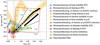 |
Fig. 3 Illustrative correlation plot for LS1 of Cell 3.1 in terms of JSC vs VOC. The figure shows how experimental and simulated correlation pathways are compared within the proposed framework. Each simulated mechanism is averaged over ≈100 simulated devices and each coloured area represents a 95% confidence interval. For degradation, the same material parameters are varied in the opposite direction (e.g. defect healing becomes defect formation). The black arrow indicates the sense of performance increase, towards higher VOC and JSC. The full mechanism list is given in the legend, grouped by layer: yellow for perovskite, blue for HTL, purple for ETL, orange for interfaces, and green for parasitic resistances. The square and polygon drawn in the plot illustrate the scoring regions: trajectories within the polygon correspond to good agreement, those within the square but outside the polygon to moderate agreement, and those outside the square to poor agreement. |
3 Results
Hereafter, the analysis of the data and results are presented for selected devices. The same procedure is applied to all cells studied. Input properties used in the model are presented in Table S2 and have been adapted from literature [13–18] or characterized experimentally. While some parameters remain constant, others are varied to simulate the mechanisms proposed.
First, the experimental correlation pathways of solar cells studied are shown in Figure 4. Trajectories are normalized with respect to their starting point, so they all start at (1,1) and their relative evolution is shown. The pathways represent the states that devices undergo along ageing in terms of their VOC-JSC correlation. For each solar cell simulated, LS1, LS2 and LID selected are shown together.
Curves in Figure 4 show how the cell’s degradation is mainly driven by a monotonous decrease in VOC, while JSC remains comparatively stable, showing a minor increase for some cases. Different trends are observed for LS1 and LS2 in most devices. LS1 (green) has a steeper slope in JSC-VOC than LS2 (blue), indicating a faster change in JSC relative to VOC. These observations do not necessarily imply different underlying mechanisms. Instead, they confirm that the rate of change differs between the two phases. Cell 4.1 is the only exception, as its LS1 and LS2 curves show more similar dynamics.
The genetic algorithm yields results such as those shown in Figure 5. Around 100 sets of parameters and their JV curves are obtained with the GA for the beginning of each ageing period studied. Then, distributions of simulation parameters are studied. Figure 5b shows the evolution of electrical parameters (VOC) along generation and mutation steps of the GA. As expected, the simulated VOC progressively approaches the experimental values as the GA advances.
In addition, the GA provides clues on ranges of material parameter values compatible with experimental data. For the specific case in Figure 5c, simulations indicate that higher perovskite defect densities better model the experimental JV, as seen when comparing the initial wide range of parameters explored to the values at the final step of the GA.
The shape of the post-selection distributions depends on both the parameter considered and the device studied. In some cases, the distribution shows a dominant peak as in Figure 5c. Thus, the GA concentrates solutions within a relatively constrained range because this parameter strongly influences the ability to reproduce the target JV metrics. In other cases, the post-selection distributions do not concentrate around a single dominant value but instead exhibit several peaks, often spread over a wide range. This indicates that multiple distinct parameter ranges can reproduce the experimental JV within the prescribed tolerance. In such cases, the parameter is less tightly constrained by JV data alone (i.e., different values can yield similarly good fits). Additional examples illustrating such multi-peak post-selection distributions are provided in the Supplementary material (Fig. S1).
Therefore, the GA provides insights into material parameters which are otherwise difficult to determine experimentally and can reduce the need for additional characterization. Although not all material parameters are constrained as clearly in every case, the method still helps identify which ones play a key role in reproducing the experimental JV.
This approach enables exploration of a wide material parameter space and discriminates multiple feasible configurations matching the experimental data. Since no single optimal solution exists for fitting a JV curve, analysing multiple combinations and their statistics prevents the limitations of adjusting parameters for an individual fit. Although further iterations of the GA can lead to an even closer agreement with experimental data, this procedure already provides sufficient information to assess the feasibility of different mechanisms. Figure 5a shows a set of JV curves that closely follow the experimental one, but do not necessarily align perfectly. This may indicate that some additional phenomena, such as the presence of ions, need to be accounted for to fully reproduce the JV characteristics.
From the outcome of the GA, LS and LID are simulated by varying a single material parameter. Around 100 different responses are computed, and the average is calculated to obtain a mapping between material and electric parameters. Figure 6 represents the case for LID related to the formation of deep defects in the perovskite, reduction of hole mobility in the perovskite, and increase of external series resistance.
Simulated mechanisms generally span experimental variation in electrical parameters. For LS1 and LS2, the variation in JSC is not always fully captured. Modelling JV curves of a degraded state from which a device performance increases proves more complex than modelling degradation starting from a higher-efficiency JV. For this reason, a reverse “pseudo-degradation” simulation from the endpoint back to the initial state was performed to reproduce the experimental JSC variation and help discriminate the dominant mechanisms.
Figure 3 in methodology presented a representative example of how the scoring framework distinguishes closely aligned, partially aligned, and clearly diverging simulated pathways. Table 1 summarises all results for LS1, LID, and LS2 of all devices studied using the score metric defined in Section 2.3.3.
Across the five analysed devices, the highest aggregated scores are obtained for deep-defect variations in the perovskite absorber, together with doping variations in the transport layers. These mechanisms show the best overall agreement with the measured ageing trajectories across the dataset. Although the analysed devices differ in perovskite precursor preparation and initial performance, aggregation across devices is useful to identify recurrent signatures that remain compatible with the measured ageing trajectories beyond cell-specific behaviour.
Aggregated scores show both cross-regime and phase-specific signatures. Deep defects in the perovskite and ETL doping contribute in both light soaking intervals and light-induced degradation when aggregated across devices, indicating that similar parameter-change signatures can be compatible with multiple ageing regimes, although not systematically in every cell. By contrast, changes in defect density at the perovskite/ETL interface are identified during LS1 and LS2, but not during LID, suggesting a more phase-specific signature within the present dataset. HTL doping also contributes across the dataset, but its contribution in LID is weaker than that of ETL doping.
In addition, variations in hole mobility in the perovskite and in defect densities at the perovskite/HTL interface can also reproduce the experimental evolution in some cases, although less consistently than the mechanisms discussed above.
Several tested candidates consistently receive low scores, including changes in electron mobility in the perovskite, electron and hole mobilities in the transport layers, and series resistance. Within the present framework, these mechanisms are therefore unlikely to be dominant drivers of the observed trajectories. This discriminatory aspect of the scoring is important, as it helps narrow the set of plausible explanations rather than only ranking compatible ones.
Table 1 should be interpreted at two levels. First, for a given mechanism, higher aggregated scores indicate more consistent agreement between simulated and experimental trajectories across devices and ageing phases. Second, at the level of an individual cell, the presence of several matching mechanisms does not necessarily imply better modelling. Instead, it may indicate greater degeneracy, with different parameter changes producing similar correlation pathways. Conversely, cells with fewer matching mechanisms may be more selective, meaning that their trajectories constrain the range of compatible explanations more strongly. In this sense, the total scores per cell quantify how constraining the experimental evolution is, rather than the absolute quality of the model.
The analysis also highlights substantial cell-to-cell variability. In line with the cell-level interpretation of Table 1 discussed above, no clear pattern emerges that can be directly attributed to fabrication method, and a larger dataset would be required to disentangle cell-specific fabrication effects from general trends and to identify systematic patterns across LS1, LID, and LS2.
These results should be interpreted within the scope of the present steady-state drift-diffusion framework. In particular, the simulations do not explicitly resolve charge-displacement dynamics such as mobile-ion redistribution or slow shallow trapping/de-trapping. Nevertheless, such processes may still contribute to the experimentally observed JV evolution and might therefore be indirectly captured through the effective parameter changes, particularly those involving the apparent doping of transport layers and the defect densities of the perovskite bulk and the perovskite/transport-layer interfaces. The mechanisms identified in this work should therefore be viewed as parameter-change signatures that best reproduce the measured JV evolution and indicate which device layers or interfaces are most consistently associated with the observed ageing trajectories, rather than as unique microscopic physical assignments.
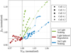 |
Fig. 4 Normalized VOC-JSC experimental correlation pathways of solar cells during ageing, smoothed along time and anchored at (1,1). Line colours denote the type of evolution: LS1 (green), LS2 (blue), LID (red). Marker shapes identify each cell as in the legend. Device labels follow the split-group notation defined in Table S1. |
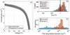 |
Fig. 5 (a) Representation of the experimental JV curve (black dashed lines) and the 99 simulated JV curves (grey) after the 8th step of the GA for LS2 of Cell 3.1. (b) Distributions of VOC at different stages of the GA. As new sets are generated, electrical parameters evolve towards the experimental value (vertical black line). (c) Example of material parameters distribution for the defects in the perovskite layer. Analysing the material parameter distribution at the end of the GA can offer insights into parameters that may be unknown or not easily measured experimentally. |
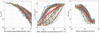 |
Fig. 6 Evolution of VOC, JSC, and FF for simulated degradation mechanisms among the cells studied. (a) Formation of deep defects in the perovskite, (b) reduction of hole mobility in the perovskite, (c) increase of series resistance. For each case, ∼100 evolutions are simulated. The average is shown in red, and the shaded area represents the 95% confidence interval. The isolated spike in panel (c) arises from a single simulation (numerical artefact) and does not affect the mean trend. |
Summary of agreement scores between experimental correlation pathways and simulated mechanisms for the five devices analysed. For each device, three adjacent columns report the scores for first light soaking (LS1), light-induced degradation (LID), second light soaking (LS2). Scores are computed as described in Section 2.3.3 and take discrete values (0, 1, 2, or 4) corresponding to increasing agreement between simulated and experimental pathways. For each mechanism and interval, the final score is obtained from considering both JSC-VOC and FF-VOC correlation pathways. Device labels follow the split-group nomenclature defined in Section 2.1, column shading indicates split groups, and the corresponding processing conditions are summarised in Table S1. The rightmost columns report aggregated scores across devices for each phase and the overall total.
4 Conclusion and outlook
In this study, we developed a framework to analyse instability pathways in perovskite solar cells by combining time-resolved JV ageing data, drift-diffusion simulations, a genetic algorithm, and correlation-pathway analysis. By comparing experimental and simulated trajectories in terms of VOC, JSC, and FF evolution, the method provides a structured way to assess which simulated mechanisms are most compatible with the measured ageing behaviour.
Across the five analysed devices, the most recurrent compatible signatures are deep-defect variations in the perovskite absorber together with doping changes in the transport layers. Some mechanisms, particularly those related to deep defects in the perovskite and ETL doping, show compatibility with both light soaking and light-induced degradation intervals across the dataset, indicating that similar parameter-change signatures can be associated with multiple ageing regimes, although not systematically in every cell. By contrast, several candidates, such as changes in transport-layer mobility, perovskite electron mobility, and series resistance, show consistently low compatibility and are therefore unlikely to be dominant drivers under the present protocol. More broadly, the proposed approach helps rank compatible parameter-change signatures and narrow the set of plausible explanations for the observed ageing trajectories.
These findings should be interpreted within the scope of the steady-state drift-diffusion framework. In the present implementation, mechanisms are simulated independently, whereas the experimental behaviour is likely governed by combinations of mechanisms acting simultaneously, and dynamic charge-transfer effects are not explicitly resolved. The identified mechanisms should therefore be regarded as effective parameter-change signatures consistent with the measured JV evolution rather than as unique physical assignments. Likewise, the limited number of devices per split condition does not allow statistically robust conclusions linking processing variations to specific mechanisms. Nevertheless, the present study demonstrates that the framework can be applied consistently to experimental ageing data and can rank parameter-change signatures associated with both performance increase and decline, highlighting the layers or interfaces most consistently linked to the observed electrical trends.
Future work should apply the framework to larger sets of similarly characterised devices to test the robustness of the trends identified here. Complementary measurements could further help constrain ion- and trap-related dynamics and refine the physical interpretation of the electronic signatures identified by the present JV-based approach. Although extending the analysis beyond the current steady-state formulation could provide a more direct link to the underlying physical origin, such modelling would come at a substantial computational cost. In this context, an important next step will be to identify a practical balance between readily accessible electrical measurements and the additional experimental or modelling complexity required for deeper mechanistic resolution.
Acknowledgments
The authors thank the IPVF fabrication team for providing the devices and associated experimental data used in this study.
Funding
This project was supported by the French Government in the Frame of the Program of Investment for the Future (Programme d’Investissement d’Avenir – ANR-IEED-002-01).
Conflicts of interest
The authors declare that they have no conflict of interest.
Data availability statement
The dataset supporting the findings of this study is available from the corresponding author upon reasonable request.
Author contribution statement
G.A.P., J.B.P., and J.F.G. designed the study. G.A.P. analysed the data, performed the simulations, and drafted the article. K.M. designed and carried out the experiments, acquired the data and contributed to the revision of the manuscript. A.J. provided guidance on the simulation framework and its application to the devices and contributed to the revision of the manuscript. J.B.P. and J.F.G. discussed the simulations and results, supervised the work and proofread the manuscript.
Supplementary Material
Figure S1: Example of multi-peak post-selection parameter distributions obtained with the GA for LS2 of Cell 3.1. Histograms comparing the initial population (blue) with the retained solutions after selection (orange) for perovskite electron mobility (top) and hole mobility (bottom). The selected distributions exhibit several peaks, indicating that multiple distinct parameter ranges can reproduce the experimental JV metrics within the prescribed tolerance. In such cases, the parameter is less tightly constrained by JV data alone than for parameters showing a single dominant peak.
Table S1: Device affiliation to split groups and inclusion in the analysis. Groups are defined by perovskite precursor preparation: solution timing (D0: prepared the same day; D-1: prepared one day in advance) and preheating prior to deposition (70 °C for 1 h vs none). Devices excluded from the analysis due to early failure or erratic measurement behaviour are identified in the table.
Table S2: Parameter inputs used for simulations of the devices studied. Fixed values have been obtained from experimental measures or the literature ([13,18]), while material parameter ranges present the values explored for LS and LID mechanisms. ETL and HTL stand for electron and hole transport layer, CB and VB for conduction and valence band, respectively.
Access Supplementary MaterialReferences
- International Energy Agency, Net zero by 2050: a roadmap for the global energy sector (IEA, Paris, May 2021). Available: https://www.iea.org/reports/net-zero-by-2050 [Google Scholar]
- International Energy Agency, World energy outlook 2023 (IEA, Paris, Oct. 2023). Available: https://www.iea.org/reports/world-energy-outlook-2023 [Google Scholar]
- M.A. Green, E.D. Dunlop, M. Yoshita et al., Solar cell efficiency tables (version 64), Prog. Photovolt. Res. Appl. 32, 425 (2024). https://doi.org/10.1002/pip.3831 [Google Scholar]
- C.C. Boyd, R. Cheacharoen, T. Leijtens, M.D. McGehee, Understanding Degradation Mechanisms and Improving Stability of Perovskite Photovoltaics, Chem. Rev. 119, 3418 (2019). https://doi.org/10.1021/acs.chemrev.8b00336 [Google Scholar]
- S.P. Dunfield et al., From defects to degradation: a mechanistic understanding of degradation in perovskite solar cell devices and modules, Adv. Energy Mater. 10, 1904054 (2020). https://doi.org/10.1002/aenm.201904054 [Google Scholar]
- W. Nie et al., Light-activated photocurrent degradation and self-healing in perovskite solar cells, Nat. Commun. 7, 11574 (2016). https://doi.org/10.1038/ncomms11574 [Google Scholar]
- O. Zbinden, E. Knapp, W. Tress, Identifying performance limiting parameters in perovskite solar cells using machine learning, Sol. RRL 8, 2300999 (2024). https://doi.org/10.1002/solr.202300999 [Google Scholar]
- A. Julien et al., Distinction of mechanisms causing experimental degradation of perovskite solar cells by simulating associated pathways, Energy Environ. Sci. 16, 190 (2023). https://doi.org/10.1039/D2EE03377A [Google Scholar]
- J. Thiesbrummel, S. Shah, E. Gutierrez-Partida et al., Ion-induced field screening as a dominant factor in perovskite solar cell operational stability, Nat. Energy 9, 664 (2024). https://doi.org/10.1038/s41560-024-01487-w [Google Scholar]
- W. Veurman, J. Kern, L. Pflüger, H. Wagner-Mohnsen, M. Müller, P.P. Altermatt, Z. Lou, M. Stolterfoht, F. Haase, S. Kajari-Schröder, R. Peibst, Deciphering hysteresis in perovskite solar cells: Insights from device simulations distinguishing shallow traps from mobile ions, Sol. Energy 284, 113037 (2024). https://doi.org/10.1016/j.solener.2024.113037 [Google Scholar]
- V.M. Le Corre, J. Diekmann, F. Peña-Camargo, J. Thiesbrummel, N. Tokmoldin, E. Gutierrez-Partida, K.P. Peters, L. Perdigón-Toro, M.H. Futscher, F. Lang, J. Warby, H.J. Snaith, D. Neher, M. Stolterfoht, Quantification of efficiency losses due to mobile ions in perovskite solar cells via fast hysteresis measurements, Sol. RRL, 6, 2100772 (2022). https://doi.org/10.1002/solr.202100772 [Google Scholar]
- M. Burgelman, P. Nollet, S. Degrave, Modelling polycrystalline semiconductor solar cells, Thin Solid Films 361–362, 527 (2000). https://doi.org/10.1016/S0040-6090(99)00825-1 [CrossRef] [Google Scholar]
- A. Slami, M. Bouchaour, L. Merad, Numerical study of based perovskite solar cells by SCAPS-1D, Int. J. Energy Environ. 13, 17 (2019). https://www.naun.org/main/NAUN/energyenvironment/2019/a082011-000.pdf [Google Scholar]
- F. Jannat, S.U. Ahmed, M.A. Alim, Performance analysis of cesium formamidinium lead mixed-halide based perovskite solar cell with MoOx as hole transport material via SCAPS-1D, Optik 228, 166202 (2021). https://doi.org/10.1016/j.ijleo.2020.166202 [Google Scholar]
- P. Yadav et al., Exploring the performance limiting parameters of perovskite solar cell through experimental analysis and device simulation, Sol. Energy 122, 773 (2015). https://doi.org/10.1016/j.solener.2015.09.046 [Google Scholar]
- J. Haddad et al., Analysing interface recombination in lead-halide perovskite solar cells with organic and inorganic hole-transport layers, Adv. Mater. Interfaces 7, 2000366 (2020). https://doi.org/10.1002/admi.202000366 [Google Scholar]
- Y.H. Khattak, F. Baig, A. Shuja, S. Beg, B.M. Soucase, Numerical analysis guidelines for the design of efficient novel n-i-p structures for perovskite solar cell, Sol. Energy 207, 579 (2020). https://doi.org/10.1016/j.solener. 2020.07.012 [Google Scholar]
- J. Peng et al., Nanoscale localized contacts for high fill factors in polymer-passivated perovskite solar cells, Science 371, 390 (2021). https://doi.org/10.1126/science.abb8687 [Google Scholar]
Cite this article as: Guillem Álvarez Pérez, Karim Medjoubi, Arthur Julien, Jean-Baptiste Puel, Jean-François Guillemoles, Simulation-based insights into light soaking and light-induced degradation in perovskite solar cells, EPJ Photovoltaics 17, 22 (2026), https://doi.org/10.1051/epjpv/2026014
All Tables
Summary of agreement scores between experimental correlation pathways and simulated mechanisms for the five devices analysed. For each device, three adjacent columns report the scores for first light soaking (LS1), light-induced degradation (LID), second light soaking (LS2). Scores are computed as described in Section 2.3.3 and take discrete values (0, 1, 2, or 4) corresponding to increasing agreement between simulated and experimental pathways. For each mechanism and interval, the final score is obtained from considering both JSC-VOC and FF-VOC correlation pathways. Device labels follow the split-group nomenclature defined in Section 2.1, column shading indicates split groups, and the corresponding processing conditions are summarised in Table S1. The rightmost columns report aggregated scores across devices for each phase and the overall total.
All Figures
|
Fig. 1 Temporal evolution of the output power for the five solar cells studied under continuous illumination at 100 mW/cm2. Light soaking (LS1, LS2) and light-induced degradation (LID) phases are observed. LS1 starts at t = 0 h, LS2 at t = 452 h after light was interrupted for 12 h, and LID occurs between them. Device labels follow the notation defined in Table S1. |
| In the text | |
|
Fig. 2 Temporal evolution of the PCE, VOC, JSC, and FF for Cell 1.2 during the first 600 h. LID happens between LS1 and LS2, LS2 occurs at t = 452 h after light interruption. Notably, simultaneous performance increase and decline are selected across all parameters, reducing the complexity of feasible mechanisms behind instabilities and making the results interpretable. An identical selection and processing procedure was applied to all cells studied. |
| In the text | |
|
Fig. 3 Illustrative correlation plot for LS1 of Cell 3.1 in terms of JSC vs VOC. The figure shows how experimental and simulated correlation pathways are compared within the proposed framework. Each simulated mechanism is averaged over ≈100 simulated devices and each coloured area represents a 95% confidence interval. For degradation, the same material parameters are varied in the opposite direction (e.g. defect healing becomes defect formation). The black arrow indicates the sense of performance increase, towards higher VOC and JSC. The full mechanism list is given in the legend, grouped by layer: yellow for perovskite, blue for HTL, purple for ETL, orange for interfaces, and green for parasitic resistances. The square and polygon drawn in the plot illustrate the scoring regions: trajectories within the polygon correspond to good agreement, those within the square but outside the polygon to moderate agreement, and those outside the square to poor agreement. |
| In the text | |
|
Fig. 4 Normalized VOC-JSC experimental correlation pathways of solar cells during ageing, smoothed along time and anchored at (1,1). Line colours denote the type of evolution: LS1 (green), LS2 (blue), LID (red). Marker shapes identify each cell as in the legend. Device labels follow the split-group notation defined in Table S1. |
| In the text | |
|
Fig. 5 (a) Representation of the experimental JV curve (black dashed lines) and the 99 simulated JV curves (grey) after the 8th step of the GA for LS2 of Cell 3.1. (b) Distributions of VOC at different stages of the GA. As new sets are generated, electrical parameters evolve towards the experimental value (vertical black line). (c) Example of material parameters distribution for the defects in the perovskite layer. Analysing the material parameter distribution at the end of the GA can offer insights into parameters that may be unknown or not easily measured experimentally. |
| In the text | |
|
Fig. 6 Evolution of VOC, JSC, and FF for simulated degradation mechanisms among the cells studied. (a) Formation of deep defects in the perovskite, (b) reduction of hole mobility in the perovskite, (c) increase of series resistance. For each case, ∼100 evolutions are simulated. The average is shown in red, and the shaded area represents the 95% confidence interval. The isolated spike in panel (c) arises from a single simulation (numerical artefact) and does not affect the mean trend. |
| In the text | |
Current usage metrics show cumulative count of Article Views (full-text article views including HTML views, PDF and ePub downloads, according to the available data) and Abstracts Views on Vision4Press platform.
Data correspond to usage on the plateform after 2015. The current usage metrics is available 48-96 hours after online publication and is updated daily on week days.
Initial download of the metrics may take a while.