| Issue |
EPJ Photovolt.
Volume 17, 2026
|
|
|---|---|---|
| Article Number | 13 | |
| Number of page(s) | 14 | |
| DOI | https://doi.org/10.1051/epjpv/2026002 | |
| Published online | 17 March 2026 | |
https://doi.org/10.1051/epjpv/2026002
Original Article
Clipping-corrected performance ratio: a new metric for high DC:AC ratio PV systems
1
National Physical Laboratory, Teddington TW11 0LW, UK
2
Statkraft UK Ltd., 19th Floor, 22 Bishopsgate, London EC2N 4BQ, UK
* e-mail: This email address is being protected from spambots. You need JavaScript enabled to view it.
Received:
18
August
2025
Accepted:
6
January
2026
Published online: 17 March 2026
Abstract
The most established key performance indicator for (PV) system performance is the performance ratio (PR) metric, which is the ratio of the actual to the expected specific yield of a PV system. Accurate PR calculations are crucial for the PV systems industry, as errors can potentially lead to hidden underperformance, unfair financial penalties and uncertainty in system value. In systems with high DC:AC ratios, the regular occurrence of inverter clipping causes problems with PR assessment which include masking degradation and increased seasonal variation. A common practice is to exclude clipped data from PR calculations, but this can bias the remaining dataset and masks problems with inverters. In this work, a new improved clipping-corrected PR (CCPR) metric is introduced and evaluated. CCPR takes into account clipping and weather variability, and allows the use of all datapoints during a PV system’s operation. We introduce the new metric and evaluate it for different locations around the world using synthetic data. Different types of clipping ratios and faults of the system are tested, demonstrating that the new PR metric is more robust compared to the current standardized PR metrics, and is not affected by weather conditions. In addition, we show that the new metric is robust against the use of low temporal resolution Typical Meteorological Year data for calculating expected PR, in contrast with standard PR metrics. The widespread adoption and potential standardization of this new metric can lead to more accurate PR assessment for PV systems, reduced contractual risks for companies in the sector and increased in confidence of PV generation by consumers.
Key words: Photovoltaic systems / performance ratio / simulations / performance assessment
© J.C. Blakesley et al., Published by EDP Sciences, 2026
 This is an Open Access article distributed under the terms of the Creative Commons Attribution License (https://creativecommons.org/licenses/by/4.0), which permits unrestricted use, distribution, and reproduction in any medium, provided the original work is properly cited.
1 Introduction
In the rapidly growing solar photovoltaics (PV) systems industry, many critical decisions are based on a few system-level performance metrics. One of the most commonly used metrics for PV system performance assessment is the performance ratio (PR), the ratio of the actual yield to the reference (nameplate) yield of a PV array or system [1]. Accurate PR calculation is crucial for the assessment of present and future finances of a PV system, as a Key Performance Indicator (KPI) used in contracts for performance guarantees and obligations [1].
The simplicity and transparency of PR makes it ideal for a performance guarantee. PR has been harmonized in international standards (IEC 61724-1 [2]), widening its acceptance in legal contracts. However, this simplicity also introduces inaccuracies [3]. One such issue is that PR is dependent on weather, particularly temperature, leading to seasonal and year-on-year variations in measured PR [4]. Corrections for temperature effects on PR calculations are described in the latest edition of the IEC 61724-1 standard and are widely used. Inaccuracies in PR calculation can lead to financial penalties for PV system companies, including developers, owners or operators. Inaccuracy and variability can also lead to uncertainty in the valuation of a system, adding risk to developers and buyers, and affects derived KPIs such as Performance Loss Rate.
When a solar PV system is designed, its performance is modelled using historical data or typical meteorological year (TMY) data. The modelling provides an estimate of the expected PR (expected yield divided by reference yield) of the system including expected losses. The model output is used in investment decisions and contract negotiations on the construction or sale of PV systems. Once a system is built, the actual PR is measured. Ideally the measured PR will match the expected PR, although, in reality, the measured PR will be different due to several factors, such as:
Underperformance of the system.
Model inaccuracy and errors in input parameters defining the PV system and site for the model used to predict expected PR. This includes overrating module power.
The weather during the measurement period is different to the weather used to model the expected PR.
Errors in measurement of the actual PR.
Data quality issues.
PR measurement is primarily for identifying poor performance of a system due to faults or other quality issues. It also offers protection against overoptimistic modelling, in which the efficiencies of system components are overestimated. The remaining 3 factors listed above should be minimized in PR measurements. Weather conditions during the measurement period strongly affect PR measurements. If the actual weather is not similar to the weather data used to model expected PR, then there may be significant errors in PR calculations. These effects become more extreme if measurement periods of less than 1 yr are used, although it is beneficial to the industry to complete contracts on shorter timescales.
A further issue with PR metrics is the effect of inverter clipping in systems with high DC:AC ratios. These are systems where the rated DC capacity of the installed PV modules exceeds the maximum AC output of the inverters. Such systems are common and have several benefits, such as supplying more constant power to the grid, or complying with a limited grid connection capacity. Inverter clipping occurs in high DC:AC systems when irradiance is high enough that the available DC output of an array is higher than the capacity of its inverter. At these times, the inverter limits the power output of the array to the inverter limit and inducing a “clipping loss”.
Clipping losses are considered in the design process of a PV system and included when modelling the expected PR. Nevertheless, the clipping losses, and therefore PR, may be overestimated or underestimated if the actual weather differs from the modelled weather. For instance, a higher-than-average number of sunny days during the reporting period results in excess unexpected clipping losses and a lower measured PR value. The current IEC 61724-1 standard does not include any correction for clipping losses in PR metric evaluation. A common practice is to filter out periods of inverter clipping from the reported PR calculations [5], thereby estimating the value of PR without clipping losses. However, as we demonstrate below, this can remove large portions of relevant performance data and introduces new problems such as masking underperformance of inverters and creating a dependence of expected PR on model time resolution [6].
In this paper we introduce a new performance metric “clipping corrected performance ratio” (CCPR). The aim of this metric is to reduce the seasonal and interannual variation in PR due to clipping. We simulate PV systems in a range of climates to generate synthetic PR measurements that we use to demonstrate the performance of the new metric in terms of interannual variation and sensitivity to system abnormalities. In Section 2 we introduce the new performance metric and our analysis methods. In Section 3 we present the results of our study. In Section 4 we present conclusions and a discussion of the limitations of our methods and further work needed. Table 1 provides a glossary of symbols used in this work.
2 Methods
2.1 Standard performance ratios
The international standard IEC 61724-1 defines several performance metrics for solar PV systems [2]. All metrics use measured timeseries data, including power output and plane of array irradiance recorded at regular intervals over a reporting period. For example, records at 15 min intervals for a period of 1 yr. From these data the measured system yield is compared against the reference system yield, calculated for the measured weather conditions, to deliver a dimensionless metric.
The standard performance metrics are grouped into performance ratios and performance indices. Performance ratios are based on simple formulae; they are easy to calculate but omit many known factors that influence system performance. On the other hand, performance indices are model based metrics that involve simulating all aspects of a system using measured weather data and comparing the actual output to modelled output. While performance indices are potentially more powerful, their complexity and reliance on third party modelling software, introducing concerns about reproducibility and traceability, are a barrier to use in performance guarantees and contractual arrangements. For these reasons, simple performance ratios are more widely used in contracts. IEC 61724-1:2021 defines two versions of a temperature corrected performance ratio (TCPR): the “25 °C performance ratio” and the “Annual-temperature-equivalent performance ratio”. In this work, we define TCPR as the former, which for monofacial systems is:
 (1)
(1)
where Pout,k is the system power output recorded at timepoint k, τk is the duration of the kth recording interval, P0 is the DC capacity of the system, which is the sum of DC power ratings of all installed modules under standard test conditions (STC) of 25 °C and irradiance Gref = 1000 W m‒2, GPOA,k is the irradiance measured in the PV modules’ plane of array and C25°C,k is a temperature correction factor:
 (2)
(2)
where γ is the relative power temperature coefficient of the PV modules and Tmod,k is the module temperature at the kth timepoint. For performance guarantees, Tmod,k is not measured directly but is estimated from the measured meteorological data with the same thermal model used in the simulation that set the performance guarantee. The thermal model is commonly a simple steady-state heat-transfer model [7,8]. Thus, PR′25°C corrects for variations in ambient temperature in a simple and transparent way. Using the alternative annual-temperature-equivalent performance ratio instead of the 25 °C performance ratio introduces an offset into PR values, but does not significantly change the results or conclusions of this work.
For bifacial systems, the rear-side plane of array irradiance  should also be measured or estimated and included in the performance ratio:
 (3)
(3)
where φ is the module power bifaciality reported on module datasheets.
2.2 Clipping corrected performance ratio
Our proposed new metric for clipping-corrected performance ratio (CCPR) is as follows: In the above temperature corrected performance ratio, the irradiance term is replaced with a clipping corrected irradiance term CCC,k; equation (1) is replaced by:
 (4)
(4)
CCC,k is equal to the POA irradiance when the temperature corrected irradiance is below a clipping threshold irradiance GC,25°C, but is independent of irradiance above this threshold:
 (5)
(5)
This behaviour is illustrated in Figure 1. For bifacial systems, GPOA,k in equation (5) is replaced with  , as with standard PR metrics. This simple approach represents the expectation that no additional power is generated for irradiances above the clipping threshold. It has the advantage of simple implementation, with no requirement for clipping detection algorithms. In principle, if a system performs as expected then the measured PR is independent of the amount of time spent above the clipping limit. Nevertheless, this does depend on appropriately determining the value of GC,25°C.
2.3 Determining clipping threshold irradiance
A nuance of the CCPR metric is that, on datapoints where clipping is expected, PR’CC is inversely proportional to GC,25°C. Therefore, the chosen value of GC,25°C directly affects the measured PR’CC value for any system with clipping. It is essential that the value of GC,25°C is agreed at the same time as a target PR value is established. Typically, this will be based on modelling of a designed or as-built system using historical weather data appropriate to the location. How to choose an appropriate value of GC,25°C is a matter for discussion. In this work we use a simple algorithm designed to minimise the weather-induced variation in CCPR:
Simulate the system and record simulated Pout,k, Tmod,k and GPOA,k, and whether clipping occurred for each timepoint k.
Chose an initial guess value of GC,25°C. An appropriate first guess is
 , where PAC,0 is the AC capacity of the array.
Sum the number of timepoints N+ for which clipping occurred, but the temperature corrected irradiance
 is less than the guess value of GC,25°C.
Sum the number of timepoints N_ for which clipping did not occur, but the temperature corrected irradiance
 is greater than the threshold value of GC,25°C.
If N+>N_ then reduce the guess value of GC,25°C, or if N+ < N_ then increase the threshold value of GC,25°C. Repeat steps 3 – 5 to find the value of GC,25°C that minimises |N+-N- |.
The result of the algorithm is illustrated in Figure 2. Following this algorithm, GC,25°C is assigned a value where the timepoints that are wrongly assigned using this threshold are equally likely to be clipped or not clipped so the bias error is likely to be minimal. The above algorithm is used for the study in this paper. However, an alternative method that is potentially more robust for more complex systems is presented in the Supporting Information. The Supporting Information also includes a discussion of the impact of choosing a different value of GC,25°C.
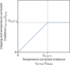 |
Fig. 1 Illustration of the behaviour of clipping and temperature corrected irradiance as a function of temperature corrected irradiance |

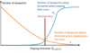 |
Fig. 2 Illustration of the selected value of GC,25°C using the method in Section 2.3. The datapoints are model outputs using historical weather data and the corrected irradiance |

2.4 Synthetic data generation
To evaluate the proposed CCPR metric, we applied it to synthetic PV systems data. Using synthetic data allowed us to compare the observed performance of a system (PR) with the true performance of a system, which is determined by simulation parameters. In a real system, only the observed performance is known, because the system can only be measured under the weather conditions that actually occur and within the limits of available instrumentation. Synthetic data also allowed us to isolate the sensitivity of the CCPR metric to environmental and system conditions, including weather variability and system underperformance.
Synthetic data were generated by a simulation model described below. The model aims to provide controllable synthetic data that are representative of systems in general, rather than an accurate model of a specific system. There are many model choices and optimizations that could have been added for greater realism, but as they are not needed for this study, we opted for a simple and general approach instead. Some specific limitations include:
The model assumes stable performance of the system – there is no degradation or any other “history” effects or time-dependent parameters (e.g. soiling) other than the weather and Sun position. Where we include failures, they are static (i.e. failed for the entire reporting period).
Perfect uniform cell temperature is assumed.
Uniform irradiance assumed across the array.
No additional site effects are included, such as shading.
All modules are identical with no variation in performance.
Inverter clipping is perfect – inverters clip at exactly the same Pac each time.
2.5 Array design
We simulated four system configurations: Fixed tilt monofacial, fixed tilt bifacial, single-axis tracker (SAT) monofacial and SAT bifacial. For each system we simulated a single inverter array representing a uniform system with identical arrays. We selected an arbitrary configuration of module and inverter: For the default monofacial configurations we used 8 strings of 24 × 300 W Canadian Solar CS6X-300M modules connected to a 36 kW Huawei SUN2000 36KTL US inverter; for default bifacial configurations we used 6 strings of 25 × 360 W Canadian Solar 1500 CS3U-360PB-FG modules connected to a 33 kW Huawei SUN2000-33KTL inverter. These gave default DC:AC capacity ratios of 1.6 and 1.57 respectively. We also simulated systems with fewer modules per string to simulate a range of DC:AC ratios from 1.6 to 0.89. Fixed-tilt arrays were aligned East-West (South-facing) and tilted at 20° and 30° for monofacial and bifacial respectively. SAT arrays were aligned North-South (rotating East to West) with optimized tilt angle.
2.6 Locations and weather data
We simulated systems using weather data and locations from a range of different climates. Weather data were acquired from the Baseline Solar Radiation Network (BSRN) [9]. Of the available sites in the BSRN database, we selected 6 locations where the data are acquired from stations located above natural surfaces, and where temperature and irradiance data are available for over 10 yr without long missing data periods. We qualified and cleaned data before use. Table 2 summarizes the chosen locations.
All weather data used in this study were recorded at 1 min intervals. By default, all calculations, including calculation of DC and AC power output and evaluation of PR metrics, were performed on timeseries using native timepoints from the BSRN weather data files. The BSRN data include global horizontal irradiance, direct normal irradiance and diffuse horizontal irradiance measurements, as well as long-wave horizontal irradiance (related to sky temperature) and ambient temperature. For each location we also produced typical meteorological year (TMY) data files at time resolutions from 1 min to 1 h. These were used to simulate the use of TMYs in estimating the expected yield and PR of a system design.
Glossary of symbols used in this paper.
Details of BSRN weather data used for this study.
2.7 Model physics
We simulated array DC and AC outputs in MATLAB by Mathworks [10] using a combination of models from PV_LIB for MATLAB [11, 12], Bifacial_radiance [13, 14], and in-house developed algorithms. The model components are summarized in Table 3.
Model components used for simulation of array DC and AC outputs.
2.8 Simulating abnormal performance
In addition to default arrays described above, we also simulated different scenarios for abnormal performance. The array definition parameters were modified to represent different types of failure, underperformance or overperformance as described in Table 4. These scenarios were used to evaluate the ability of PR metrics to identify abnormal performance.
Summary of simulated abnormal performance scenarios.
2.9 Statistical analysis
By simulating all array definitions in all locations, we performed statistical evaluations of the TCPR and CCPR metrics. For each location and each array definition we first ran a “design simulation” to simulate the expected yield of the array. The design simulation uses hourly TMY weather data and a simplified steady-state thermal model to emulate typical design simulation practices. For each array and location combination the value of GC,25°C is derived from the design simulations. Next, we performed simulations of all array types using the entire 1 min resolution weather dataset for each location to generate synthetic PV system output data. The PR metrics are evaluated for each timepoint in the simulation and for the whole weather dataset period as well as multiple 12 month intervals within each dataset. Where there were gaps in the weather data, the 12 month periods were extended so that each annual interval contains 12 months of good data.
We define the “True Performance Ratio” PRtrue for each performance ratio variant as the PR value determined from the synthetic output data generated over the whole multi-year weather dataset. There is one value of PRtrue for each combination of PR metric, location and array definition. Its value is constant over the time window of the whole dataset as our model does not include degradation. PRtrue is used as the “ground truth”; it is taken to be an estimate of “the statistical expectation of the long-term average performance ratio of a system assuming that the system condition does not change”. The “Annual Performance Ratio” PRannual is the PR value determined from a single 12 month period of synthetic data.
Ideally any value of PRannual is as close as possible to PRtrue for a given system and location. However, weather variations introduce random variations. We define a figure of merit “annual variability” as the root-mean squared error (RMSE) of PRannual compared to PRtrue:
 (6)
(6)
where PRi,j is the performance ratio of a given array evaluated over the ith 12-month period for the jth location and PRtrue,j is the True Performance Ratio for the same array and location. The annual variability is a measure of the sensitivity of a performance ratio to interannual weather variation.
To evaluate the accuracy of a PR metric for quantifying abnormal performance of a system we define two additional statistics. We define the “True Energy Performance Index”, EPItrue, as the ratio of the energy generated for the given array over the entire weather dataset for the specific location divided by the energy generated by the default array over the same period and location:
 (7)
(7)
where EPItrue,j,l is the EPItrue for the lth array definition and jth location, Pout,k,j,l is the AC output power for that array at timepoint k and Pout,k,j,default is the same for the default array definition. For an array l that is behaving abnormally according to one of the definitions in Table 4, this index is an estimate of how much energy the array will produce over a long period of time relative to an identical array that is performing exactly as expected. In other words, the EPItrue is a measure of the true quality of a system compared to its expected quality accounting for all modelled losses. For an array that is behaving as expected, EPItrue = 1. For an array with failures EPItrue is less than one. There is one value of this metric for each array and location combination.
The “Annual PR/ Expected PR” ratio PRannual/PRexpected is the ratio of the observed performance of the system compared to the expected performance. To calculate this ratio, we use PRtrue of the default array as the expected PR (PRexpected), because the default array represents the expected behavior on which performance guarantees would be based. This metric represents the ratio of the PR that is measured during a 12-month assessment compared to the modelled expected PR for a correctly performing system. If a system is underperforming, then the value of PRannual/PRexpected should be less than one. Ideally, the difference (1 - PRannual/PRexpected) should be proportional to the long-term expected energy loss due to underperformance. Therefore, PRannual/PRexpected = EPItrue is the goal for a perfect performance ratio metric. We define as second figure of merit “annual accuracy” as the RMSE between these values:
 (8)
(8)
where PRi,j,l is the PR evaluated for the lth array definition over the ith 12-month period for the jth location and PRi,j,default is the same for the default array definition. This figure of merit is an indication of how accurately the annual PR metric can identify issues in the long-term expected energy yield of the system.
3 Results
3.1 Effect of DC:AC ratio on performance ratio
Figure 3 shows the average fraction of energy that is generated under clipping conditions for the default arrays operating nominally with different DC:AC ratios in one location. Other locations are shown in the Supporting Information. In the sunniest location (IZA), about 65% of energy is generated while the inverter is clipping for a monofacial fixed-tilt array with a DC:AC ratio of 1.6. This varies by about ± 2% between different years in the data set. In this case, excluding clipped data points from the PR calculation would exclude 65% of available data and significantly bias the result toward unusually low irradiance conditions. This rises to about 85% for single-axis tracker arrays.
Figure 4 shows how the calculation of different PR metrics from the synthetic data varies as a function of DC:AC ratio for one location. Results for other locations follow similar trends and are shown in the Supplemental Information. The TCPR value is significantly impacted by DC:AC ratio as high DC:AC ratio results in significant clipping losses which are not mitigated in the PR calculation. In the most extreme case (location IZA), the TCPR changed from 94% to 73% when DC:AC ratio increased from 1.0 to 1.6. The magnitude of interannual variation in TCPR is also highest in scenarios with the most clipping. The clipping dependence of TCPR is mitigated by excluding data where clipping occurred. However, as we show in Section 3.2 below, the exclusion of data can lead to masking of abnormal behavior. Using CCPR reduces the dependence of PR on DC:AC ratio similar to excluding clipping data points. We do not show TCPR for bifacial arrays in Figure 4, though patterns were similar for both monofacial and bifacial arrays.
An example timeseries of daily PR values, shown in Figure 5, illustrates how temperature and clipping correction influence seasonal variability for a system with high DC:AC ratio. When no corrections are applied, PR drops in the summer when temperatures are high and rises in the winter when temperatures are low. Applying temperature correction flattens the winter peaks, but there is still a significant drop in PR on most summer days caused by clipping. Excluding clipped data points reduces this effect, but does not resolve it entirely. Applying clipping correction instead resolves the drop in PR over summer days. The main remaining seasonal effect is the larger scatter in daily values in winter months caused by the frequency of days with very low total irradiation.
In practice, seasonal variations are mitigated by using annual PR metrics. Nevertheless, seasonal patterns are not identical from 1 yr to another so residual weather-induced year-on-year variations in annual PR remain. The impact of choice of correction method on interannual variation in measured PR is illustrated by the annual variability metrics summarized in Table 5. For a DC:AC ratio of 1.0, most interannual variation is corrected by applying temperature correction only. However, for a DC:AC ratio of 1.6, most variation is not corrected by temperature correction, but is corrected from 0.59% to 0.15% by the addition of clipping correction. It is clear that most interannual variation is therefore due to clipping, rather than temperature in (idealized) high DC:AC ratio systems. We conclude that in high DC:AC systems clipping correction is of similar importance as temperature correction. This conclusion was true for all 4 system configurations studied.
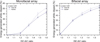 |
Fig. 3 Fraction of energy generated under clipping conditions as a function of DC:AC ratio for nominally performing systems. Error bars indicate standard deviation between different 12 month periods. Dashed lines indicate single-axis tracker systems, solid lines are fixed-tilt. For simplicity, only one location is shown here; other locations are shown in the Suporting Information. Left: monofacial array. Right: bifacial array. |
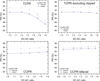 |
Fig. 4 Average (symbols) and standard deviation (error bars) of annual PR values determined for nominally performing (default) arrays as a function of DC:AC ratio for the default array in one location. Results for other locations are shown in the Supporting Information. Solid lines are fixed-tilt systems and dashed lines for single-axis trackers. Top-left: Temperature corrected PR on monofacial arrays. Top-right: The same but excluding datapoints where clipping occurs. Bottom-left: Clipping corrected PR on monofacial arrays. Bottom-right: Clipping corrected bifacial PR on bifacial arrays. |
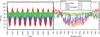 |
Fig. 5 Seasonal effects on different PR metrics illustrated by synthetic timeseries of daily PR values for the default monofaical array type with DC:AC ratio 1.6 at the PAY location. Nine years are shown in the left, year 10 is expanded on the right. Colours correspond to four variants of PR metrics: Red = uncorrected PR; blue = TCPR (Eq. (1)); yellow = TCPR where clipped data points are excluded from the PR calculation; green = CCPR (Eq. (4)). Standard deviations over the 10 yr period for each metric are displayed in the inset. |
Annual variability (Eq. (6)) for the default monofacial fixed-tilt array with different DC:AC ratios with nominal performance (no failures or degradation). Here TCPR represents the 25 °C performance ratio. The same table using annual-temperature-equivalent performance ratio is shown in the supporting information.
3.2 Sensitivity to array underperformance
Figure 6 shows the annual performance metrics measured from synthetic data for each year and each location for high DC:AC ratio arrays with different abnormal performance characteristics described in Table 4. Each annual PR value is normalized according to the expected PR (i.e. the PR value based on a design simulation with expected losses and a typical meteorological year). This is compared against the true energy performance index calculated by equation (7). For an ideal PR metric, the annual PR is proportional to the true performance of a system with minimal scatter or bias, and therefore all scatter points should lie as close as possible to the solid straight line indicated on Figure 6.
For uncorrected PR (top left), there is a strong correlation between annual PR and true performance. However, there is considerable scatter caused by interannual variation. Thus, we conclude that uncorrected annual PR is unbiased but imprecise. The TCPR metric (top right) is similarly unbiased, but still imprecise due to the interannual variation induced by clipping. Excluding clipping data from the PR calculation (bottom left) notably reduces the interannual variation. However, a bias is introduced when arrays perform abnormally. The bias is introduced as the exclusion of data weights the PR metric to conditions of low light when the array output is not clipped. This masking effect has been previously described by Balfour et al. [18] who also noted that degradation rates can be underestimated for high DC:AC ratio systems. The use of CCPR (bottom right) removes both the scatter and the bias induced by clipping. Note, however, that the masking of degradation (not simulated in this study) may still be present. The use of TCPR excluding clipped data may be most informative in quantifying performance degradation of the DC part of a system.
The annual accuracy statistic, calculated according to equation (8), reveals the limits of sensitivity of PR metrics for detecting abnormal behavior in a system. In the case that all faults are equally likely, the annual accuracy is 2.68% for a monofacial fixed tilt system with DC:AC ratio 1.6 when using TCPR excluding clipped data points. The annual accuracy falls to 0.27% when using CCPR. Using CCPR instead of TCPR provides a significant improvement in the ability to discriminate between faulty behavior versus unexpected weather. Consider a use case where a target PR value is assigned in a contract, below which a penalty must be paid. Due to the combination of weather variability and clipping, this threshold must be set somewhat below the expected PR of the system to avoid a significant probability of penalties being issued for correctly performing systems (false positives). In the case of TCPR, there is considerable overlap in annual PR values between correctly performing and defective systems. As a result, there is no threshold PR value that can avoid false positives without introducing a significant probability of false negatives. Switching to the CCPR metric enables a more selective discrimination threshold to be set. In the idealized case modelled here, setting the threshold about 1% below the expected CCPR captured 100% of failures without generating any false positives. Note that this simulation considers inverter-level PR metrics. When considering a single PR value calculated for an entire system of multiple inverters the sensitivity to a single failure diminishes proportionately. A table of annual accuracy statistics for all array types and metrics is given in the Supporting Information.
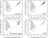 |
Fig. 6 Scatter plot of ratio of annual / expected PR versus true performance index for abnormally performing monofacial fixed-tilt arrays simulated in six different locations. Each figure shows a different variant of PR metric. Each point shows results from 1 yr at one location. Different point colors indicate arrays with different performance issues. The default array is an array that performs exactly as expected. All arrays have a DC:AC ratio of 1.6. |
3.3 Impact of model time resolution
Using low time-resolution weather data for modelling PV systems results in an underestimate of predicted clipping loss [6, 19–22]. This is because the irradiance values are typically averages over the time intervals. If an interval contains variable irradiance which is sometimes above the clipping threshold and sometimes below, but the average irradiance over the same interval is below the clipping threshold, then the system is modelled as if no clipping occurs and the system output is overestimated. In other words, the simulated weather is less variable than the real weather. It is common practice to use TMY or historical weather data with 1 h time resolution for yield estimation and setting target PR values, which can lead to an overestimation of predicted yield and PR up to about 4% for high DC:AC ratio systems. Shorter time resolutions of 30 min or 15 min are becoming more popular in modelling, but it has also been argued that the effects of random noise in high resolution satellite weather data may cancel out the benefit of using sub-hourly intervals [23]. Alternatively, several methods have been proposed to correct predicted yield and PR modelled from hourly weather data. However, these are climate specific and significant errors still remain [6, 22–26].
To simulate the response of different PR metrics to different time resolutions used for design simulations, we aggregated 1 min BSRN weather data into longer time intervals from 2 min to 1 h and repeated the system simulations. The resulting PR metrics averaged across all sites are shown in Figure 7. Using the TCPR metric, we observed as expected that the modelled PR increased continuously for high DC:AC ratio systems with increasing interval time from 1 min to 1 h. Excluding clipped data from the TCPR metric greatly reduces the impact of this effect. However, as we discuss below, this introduces a requirement for high time-resolution monitoring. Applying the CCPR metric also removes the dependence of modelled PR on model time resolution.
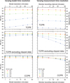 |
Fig. 7 Left: Variation of modelled PR with model time resolution based on aggregation of 1 min resolution weather data into longer time intervals. Right: Variation of measured PR with measurement time resolution based on simulating the effect of aggregating 1 min resolution sensor and system outputs into longer time intervals. PR metrics are averaged over 6 BSRN locations for the default monofacial fixed-tilt system. Different colors represent different DC:AC ratios. |
3.4 Impact of PR measurement frequency
IEC 61724-1:2021 defines requirements of sensors and sampling for PV system monitoring data [2]. The standard recommends that irradiance and weather data are recorded at 1 min intervals, with each record being an average of measurements taken at sampling intervals of 5 s or less. However, the standard allows “medium accuracy” class B monitoring with recording intervals up to 15 min and sampling intervals up to 1 min. In practice, a range of recording intervals are used with 5 min and 15 min intervals anecdotally being common.
In principle, the aggregation of measurement data to lower time resolutions does not affect uncorrected measured PR values. However, corrections for temperature and clipping introduce non-linearities to the PR equation which can distort PR values when the recording interval approaches the timescale of temperature or irradiance variations respectively. To simulate this effect, we simulated systems at 1 min resolution, but aggregated the output data (Pout,k, Tamb,k, GPOA,k) at longer intervals from 2 min to 1 h. The PR metrics were then calculated based on these lower resolution outputs. The results are shown on the right of Figure 7. For the TCPR metric, increasing the monitoring resolution introduces a very small bias that only becomes significant at recording intervals of 30 min or greater. However, when clipped datapoints are excluded from the PR metric the measured PR drops by about 3.5% as the interval is increased from 1 min to 1 h. This is because there are many 1 h intervals in which the output power is reduced by intermittent clipping but the average irradiance over the interval is below the threshold for clipping to be detected. The outcome would also depend on the method of clipping detection [27]. We used a simple power threshold on Pout,k to filter out clipped data. On using CCPR there still remains a significant dependence of recording interval of about half the magnitude of TCPR excluding clipped data. Thus, it is still important in monitoring systems with high DC:AC ratios to calculate PR at high frequencies to avoid underreporting PR values. Note that the effect is still not saturated between 1 min and 2 min intervals, which suggests that there may be benefit to using recording intervals of even less than 1 min.
4 Conclusions
Inverter clipping significantly distorts standard performance ratio (PR) performance indicators. Excluding clipped data points from the PR evaluation reduces this distortion but risks masking underperformance. We introduced a new clipping corrected performance ratio (CCPR) that removes this distortion without data loss. Using synthetic PV systems data based on real weather data we showed that the new metric, which corrects for clipping and temperature effects, had less annual variability and better accuracy that standard temperature corrected performance ratios (TCPR). We drew the following conclusions from statistical analysis of the simulation outputs:
In high DC:AC ratio systems, correcting for clipping is of similar importance as correcting for temperature in terms of reducing weather-induced PR variability.
Interannual variability of PR is reduced by excluding clipped data from the TCPR calculation or using the new CCPR metric.
Excluding clipped data from a TCPR metric introduces biases into measured PR that can mask or accentuate different failure or degradation modes of solar PV systems. This can have a critical impact at the system commissioning phase, where the PR of the system is measured and compared with expected PR from the design phase of a PV system project.
Of the PR metrics tested, CCPR offers the best accuracy for determining current system performance relative to expected performance.
For high DC:AC ratio systems, the use of hourly weather data in simulations can lead to an overestimate of expected standard PR metrics as the clipping losses are underestimated compared to 1 min resolution weather data. Using the CCPR metric eliminates this effect.
When measuring PR in high DC:AC ratio systems, the recording interval time has an important impact on the ability to filter or correct for clipping events. This can lead to significant negative error in the reported PR. The calculation of CCPR using 1 min intervals is recommended for these systems to mitigate this effect.
The above findings highlight that the CCPR can be a significant improvement for accurate performance assessment of solar PV systems, and can become the preferred metric used in contracts. Overall, we found that the CCPR approach presented in this work is simple to implement yet effective at mitigating weather dependent clipping variability in PR measurements. Adoption of the new CCPR metric can have a direct impact on future revisions of IEC 61724-1, and can result in lower risks of investment in the solar PV system industry, leading to increased bankability of solar PV projects and a consequent increase in deployment and investment in renewable energy. We would advise the use of a CCPR performance indicator in all systems where clipping is expected to occur, or where the DC:AC ratio is greater than 1.0. While the new CCPR metric better reflects system energy performance, clipping in high DC:AC systems may still mask the early effects of module degradation. For this reason, it may not be suited to certain analyses, such as performance loss rate analysis, where TCPR based on DC power excluding clipped data points may work best. It is likely that CCPR will be most useful alongside, rather than instead of, other metrics.
Our approach used synthetic data generated for simple model systems that allowed us to isolate the effect of weather variability on PR metrics from the many other correlated phenomena in PV systems. Indeed, this is the only way to perform such an experiment since weather cannot be controlled in real systems. In reality, however, there are additional effects that can influence the real measured PR values such that real annual variability values will be higher than those presented here. We have only considered a single array configuration for each array type in this work; we cannot quantify the extent to which the specific results can be generalized to any system topography and PV module or inverter technology. The model results are much more “perfect” than real world data. Real-world interannual variation is much higher due to soiling, shading, systems availability, maintenance, degradation and failures. Finally, we have not included measurement uncertainties, data quality issues, or model input parameter uncertainties, which exist for real systems and datasets. Hence, we would urge the academic community and industry to apply and trial the new metric with field datasets from real PV systems, to get insights on the performance of the metric and potential adoption in IEC 61724-1.
Acknowledgements
The authors thank Lavanya Malarkannan and Spencer Thomas of the National Physical Laboratory for reviewing this paper.
Funding
This work has received funding from the UK Department for Science, Innovation and Technology through Innovate UK’s “Analysis for Innovators Round 7” programme and through the UK National Measurement System. Part of this work were carried out in the 24GRD04 SOLiD-PV project. The project (24GRD04 SOLiD-PV) has received funding from the European Partnership on Metrology, co-financed from the European Union’s Horizon Europe Research and Innovation Programme and by the Participating States.
Conflicts of interest
The authors certify that they have no financial conflicts of interest (eg., consultancies, stock ownership, equity interest, patent/licensing arrangements, etc.) in connection with this article.
Data availability statement
Data associated with this article are not disclosed due commercial and intellectual property considerations.
Author contribution statement
Conceptualization, JCB, GK, EK, GLM; Methodology, JCB, GK, EK, GLM, AP; Software, JCB, EK, GLM, AP; Validation, JB, GLM; Formal Analysis, JCB; Resources, JCB, JM; Writing – Original Draft Preparation, JCB, GK; Writing – Review & Editing, JCB, GK, EK, GLM; Funding Acquisition, JCB, GK, EK, GLM, JM.
Supplementary Material
Supplementary Material provided by the author. Access Supplementary Material
References
- Operation and maintenance best practice guidelines, 5 ed. (Solar Power Europe, 2021) [Google Scholar]
- IEC 61724-1:2021 photovoltaic system performance part 1: monitoring, 2021 [Google Scholar]
- D. Thevenard, A. Pai, Is it time to ditch the concept of Performance Ratio?, in 2016 IEEE 43rd Photovoltaic Specialists Conference (PVSC) (2016), pp. 3193–3198 [Google Scholar]
- T. Dierauf, A. Growitz, S. Kurtz, J.L.B. Cruz, E. Riley, C. Hansen, Weather-Corrected Performance Ratio, National Renewable Energy Laboratory (NREL), Golden, CO (United States), United States (2013). https://www.osti.gov/biblio/1078057 [Google Scholar]
- S. Lindig, M. Theristis, D. Moser, Best practices for photovoltaic performance loss rate calculations, Prog. Energy Rev. 4, 16 (2022) [Google Scholar]
- R. Kharait, S. Raju, A. Parikh, M.A. Mikofski, J. Newmiller, Energy yield and clipping loss corrections for hourly inputs in climates with solar variability, in 47th IEEE Photovoltaic Specialists Conference (PVSC) (Electr Network, New York: Ieee, 2020), pp. 1330–1334 [Google Scholar]
- Array Thermal losses. https://www.pvsyst.com/help-pvsyst7/index.html?thermal_loss.htm [Google Scholar]
- D. Faiman, Assessing the outdoor operating temperature of photovoltaic modules, Prog. Photovolt.: Res. Appl. 16, 307 (2008) [CrossRef] [Google Scholar]
- A. Driemel et al., Baseline surface radiation network (BSRN): structure and data description (1992–2017), Earth Syst. Sci. Data 10, 1491 (2018) [Google Scholar]
- MATLAB [Google Scholar]
- J.S. Stein, W.F. Holmgren, J. Forbess, C.W. Hansen, PVLIB: Open source photovoltaic performance modeling functions for Matlab and Python, in 2016 IEEE 43rd Photovoltaic Specialists Conference (PVSC) (2016), pp. 3425–3430 [Google Scholar]
- PV_LIB Toolbox. https://pvpmc.sandia.gov/applications/pv_lib-toolbox/ [Google Scholar]
- S. Ayala Pelaez, C. Deline, Bifacial_radiance: a python package for modeling bifacial solar photovoltaic systems, J. Open Source Softw. 5, 1865 (2020) [CrossRef] [Google Scholar]
- Photovoltaic bifacial irradiance and performance modeling toolkit. https://www.nrel.gov/pv/pv-bifacial-irradiance-toolkit.html [Google Scholar]
- N. Martin, J.M. Ruiz, Calculation of the PV modules angular losses under field conditions by means of an analytical model (vol 70, pg 25, 2001), Sol. Energy Mater. Sol. Cells 110, 154 (2013) [Google Scholar]
- PVsyst photovoltaic software. https://www.pvsyst.com/ [Google Scholar]
- J. Barry et al., Dynamic model of photovoltaic module temperature as a function of atmospheric conditions, Adv. Sci. Res. 17, 165 (2020) [Google Scholar]
- J. Balfour, R. Hill, A. Walker, G. Robinson, T. Gunda, J. Desai, Masking of photovoltaic system performance problems by inverter clipping and other design and operational practices, Renew. Sustain. Energy Rev. 145, 111067 (2021) [Google Scholar]
- J.O. Allen, W.B. Hobbs, M. Bolen, The effect of short-term inverter saturation on PV performance modeling (2018). Available: https://pvpmc.sandia.gov/app/uploads/sites/243/2022/10/Jon_Allen_AtCError_PVPMC_Poster_20180427c3.pdf [Google Scholar]
- D.A. Bowersox, S.M. MacAlpine, Predicting subhourly clipping losses for utility-scale PV systems, in 48th IEEE Photovoltaic Specialists Conference (PVSC) (Electr Network, NEW YORK: Ieee, 2021), pp. 2507–2509 [Google Scholar]
- K. Anderson, K. Perry, Estimating subhourly inverter clipping loss from satellite-derived irradiance data, in 47th IEEE Photovoltaic Specialists Conference (PVSC) (Electr Network, NEW YORK: Ieee, 2020), pp. 1433–1438 [Google Scholar]
- A. Parikh, K. Perry, K. Anderson, W.B. Hobbs, R. Kharait, M.A. Mikofski, Validation of subhourly clipping loss error corrections, in 2021 IEEE 48th Photovoltaic Specialists Conference (PVSC) (2021), pp. 1670–1675 [Google Scholar]
- M.A. Mikofski, W.F. Holmgren, J. Newmiller, R. Kharait, Effects of solar resource sampling rate and averaging interval on hourly modeling errors, IEEE J. Photovolt. 13, 202 (2023) [Google Scholar]
- D. Cormode, N. Croft, R. Hamilton, S. Kottmer, A method for error compensation of modeled annual energy production estimates introduced by intra-hour irradiance variability at PV power plants with a high DC to AC ratio, in IEEE 46th Photovoltaic Specialists Conference (PVSC) (Chicago, IL, NEW YORK: Ieee, 2019), pp. 2293–2298 [Google Scholar]
- K. Bradford, R. Walker, D. Moon, M. Ibanez, Ieee, A regression model to correct for intra-hourly irradiance variability bias in solar energy models, in 47th IEEE Photovoltaic Specialists Conference (PVSC) (ELECTR NETWORK, NEW YORK: Ieee, 2020), pp. 2679–2682 [Google Scholar]
- W. Hayes, L. Ngan, M. Francis, Ieee, Improving hourly PV power plant performance analysis: irradiance correction methodology, in 39th IEEE Photovoltaic Specialists Conference (PVSC) (Tampa, FL, 2013), pp. 775–778 [Google Scholar]
- K. Perry, M. Muller, K. Anderson, Performance comparison of clipping detection techniques in AC power time series, in 48th IEEE Photovoltaic Specialists Conference (PVSC) (Electr Network, NEW YORK: Ieee, 2021), pp. 1638–1643 [Google Scholar]
Cite this article as: James Blakesley, George Koutsourakis, Elena Koumpli, Giuliano Luchetta Martins, Anastasia Panoui, Jan Muller, Clipping-corrected performance ratio: a new metric for high DC:AC ratio PV systems, EPJ Photovoltaics 17, 13 (2026), https://doi.org/10.1051/epjpv/2026002
All Tables
Annual variability (Eq. (6)) for the default monofacial fixed-tilt array with different DC:AC ratios with nominal performance (no failures or degradation). Here TCPR represents the 25 °C performance ratio. The same table using annual-temperature-equivalent performance ratio is shown in the supporting information.
All Figures
|
Fig. 1 Illustration of the behaviour of clipping and temperature corrected irradiance as a function of temperature corrected irradiance |
| In the text | |
|
Fig. 2 Illustration of the selected value of GC,25°C using the method in Section 2.3. The datapoints are model outputs using historical weather data and the corrected irradiance |
| In the text | |
|
Fig. 3 Fraction of energy generated under clipping conditions as a function of DC:AC ratio for nominally performing systems. Error bars indicate standard deviation between different 12 month periods. Dashed lines indicate single-axis tracker systems, solid lines are fixed-tilt. For simplicity, only one location is shown here; other locations are shown in the Suporting Information. Left: monofacial array. Right: bifacial array. |
| In the text | |
|
Fig. 4 Average (symbols) and standard deviation (error bars) of annual PR values determined for nominally performing (default) arrays as a function of DC:AC ratio for the default array in one location. Results for other locations are shown in the Supporting Information. Solid lines are fixed-tilt systems and dashed lines for single-axis trackers. Top-left: Temperature corrected PR on monofacial arrays. Top-right: The same but excluding datapoints where clipping occurs. Bottom-left: Clipping corrected PR on monofacial arrays. Bottom-right: Clipping corrected bifacial PR on bifacial arrays. |
| In the text | |
|
Fig. 5 Seasonal effects on different PR metrics illustrated by synthetic timeseries of daily PR values for the default monofaical array type with DC:AC ratio 1.6 at the PAY location. Nine years are shown in the left, year 10 is expanded on the right. Colours correspond to four variants of PR metrics: Red = uncorrected PR; blue = TCPR (Eq. (1)); yellow = TCPR where clipped data points are excluded from the PR calculation; green = CCPR (Eq. (4)). Standard deviations over the 10 yr period for each metric are displayed in the inset. |
| In the text | |
|
Fig. 6 Scatter plot of ratio of annual / expected PR versus true performance index for abnormally performing monofacial fixed-tilt arrays simulated in six different locations. Each figure shows a different variant of PR metric. Each point shows results from 1 yr at one location. Different point colors indicate arrays with different performance issues. The default array is an array that performs exactly as expected. All arrays have a DC:AC ratio of 1.6. |
| In the text | |
|
Fig. 7 Left: Variation of modelled PR with model time resolution based on aggregation of 1 min resolution weather data into longer time intervals. Right: Variation of measured PR with measurement time resolution based on simulating the effect of aggregating 1 min resolution sensor and system outputs into longer time intervals. PR metrics are averaged over 6 BSRN locations for the default monofacial fixed-tilt system. Different colors represent different DC:AC ratios. |
| In the text | |
Current usage metrics show cumulative count of Article Views (full-text article views including HTML views, PDF and ePub downloads, according to the available data) and Abstracts Views on Vision4Press platform.
Data correspond to usage on the plateform after 2015. The current usage metrics is available 48-96 hours after online publication and is updated daily on week days.
Initial download of the metrics may take a while.