| Issue |
EPJ Photovolt.
Volume 17, 2026
Special Issue on ‘EU PVSEC 2025: State of the Art and Developments in Photovoltaics', edited by Robert Kenny and Carlos del Cañizo
|
|
|---|---|---|
| Article Number | 8 | |
| Number of page(s) | 17 | |
| DOI | https://doi.org/10.1051/epjpv/2026001 | |
| Published online | 13 February 2026 | |
https://doi.org/10.1051/epjpv/2026001
Original Article
A comprehensive framework for accurate estimation of performance loss rates in large photovoltaic systems using machine learning
1
Kiel University of Applied Sciences, Sokratesplatz 1, 24149 Kiel, Germany
2
Fraunhofer Institute for Microstructure of Materials and Systems IMWS, Walter-Huelse-Str. 1, 06120 Halle, Germany
3
saferay Holding GmbH, Rosenthaler Str. 34/35, 10178 Berlin, Germany
4
Wattmanufactur GmbH & Co. KG, 25899 Galmsbüll, Germany
* e-mail: This email address is being protected from spambots. You need JavaScript enabled to view it.
Received:
14
July
2025
Accepted:
24
December
2025
Published online: 13 February 2026
Abstract
Accurate quantification of long-term Performance Loss Rate in photovoltaic systems is critical for ensuring system reliability, financial forecasting, and asset management across the global PV fleet. Conventional methods for estimating the performance loss rate, however, are often constrained by their sensitivity to environmental variability and reliance on rigid filtering heuristics that can introduce bias. This paper introduces a novel, data-driven framework that transcends these challenges by integrating unsupervised filtering, predictive modeling, and advanced trend analysis. The methodology employs Density-Based Spatial Clustering of Applications with Noise to adaptively isolate anomalous operational data while preserving approximately 80% of the core performance data. Subsequently, a Light Gradient Boosting Machine model, trained on early-life system data, establishes a weather-normalized performance baseline to generate a Performance Ratio Index—a high-fidelity time-series signal representing the system's intrinsic health. Finally, the degradation pathway is characterized via Seasonal-Trend decomposition combined with the Pruned Exact Linear Time algorithm, which robustly identifies change points and non-linear aging phases. The framework was validated across 8 distinct locations comprising 84 inverters, including commercial fleets and authoritative public benchmark datasets from Eurac Research and the FOSS Research Centre. While the broad fleet analysis captured a wide distribution of trend estimates (−4%/year to +3%/year) reflecting the method's sensitivity to data duration and sensor quality, the detailed primary case study demonstrated the framework's high precision, in identifying non-linear, multi-phase degradation. This analysis revealed complex aging dynamics that differed by device, including sharp initial deceleration and instances of mid-life performance acceleration. The resulting degradation rates, with both phase-specific and time-weighted averages ranging from −0.78%/year to −0.20%/year, were found to be physically plausible and consistent with reported industry benchmarks. These findings confirm the framework's utility as a scalable tool for automated performance loss rate assessment that separates non-linear degradation trends from environmental noise.
Key words: System degradation / performance ratio / light gradient boosting machine (LGBM) / density-based spatial clustering of applications with noise (DBSCAN) / machine learning
© K.-P. Cheung et al., published by EDP Sciences, 2026
 This is an Open Access article distributed under the terms of the Creative Commons Attribution License (https://creativecommons.org/licenses/by/4.0), which permits unrestricted use, distribution, and reproduction in any medium, provided the original work is properly cited.
1 Introduction
The global installed capacity of photovoltaic systems continues to expand rapidly, making solar energy a cornerstone of the transition to a sustainable energy future. Over the operational lifetime of these systems, various factors such as material fatigue and environmental conditions lead to energy losses, directly impacting profitability and asset value. Accurately quantifying this decline, expressed as the Performance Loss Rate (PLR), is therefore critical for financial modeling, warranty claims, and optimizing operations and maintenance (O&M) strategies [1–4]. The PLR does not only indicate the irreversible physical degradation of PV systems but also measures performance-reducing events, which can be reversible or preventable through good O&M practices [5,6].
The fundamental approach to PLR estimation involves comparing measured system outputs (actual values) against an expected performance baseline (target values). Historically, two main categories of models have been used to determine these target values. The first includes empirical and statistical models, which use historical data to forecast performance [7]. While computationally efficient, their accuracy is often limited by their dependence on training data and their inability to generalize to novel conditions. The second category consists of physics-based models, such as two-diode simulations, which rely on detailed electrical and thermal equations [8]. These models can be highly accurate but require extensive domain expertise and detailed component parameters that are often unavailable for commercial systems.
A primary limitation of both traditional approaches is their difficulty in modeling the complex, non-linear relationships between environmental inputs and system output. To address this, machine learning (ML) models, particularly Artificial Neural Networks (ANNs), have emerged as a powerful alternative capable of learning these non-linear dependencies directly from large operational datasets. However, as highlighted in the comprehensive IEA PVPS Task 13 report on PLR assessment [9] and failure monitoring [10], the application of ML for long-term analysis presents its own set of challenges. A central issue is data quality. The report specifically warns that conventional “heavy data filtering” based on static rules can cause a “massive amount of data removal” and “introduce strong bias” in the final results.
In terms of relevant PLR methods, the report identifies the following as the most widely used statistical approaches: seasonal and trend decomposition using LOESS (STL), year-on-year (YoY), least-squares linear regression (LS-LR), and classical seasonal decomposition (CSD). The STL method assumes a stable and well-defined seasonal pattern and high-quality, regularly sampled data [10]; weakness of changing seasonality can lead to an overestimation of the seasonal component and thus bias the extracted trend and the resulting PLR. The YoY method is highly sensitive to data accuracy and completeness, and for certain technologies (e.g., mono-Si) method-dependent biases have been observed that cannot be attributed solely to physical behavior. LS-LR assumes a linear relationship between chosen metric and time and is most appropriate when only a few predictors are considered; in practice, it is strongly affected by outliers and unmodeled non-linearities, whereas real PV time series typically violate these assumptions. CSD, in turn, is based on centered moving averages over multiple months, which leads to a systematic exclusion of the first and last months and depends on data and requires an appropriate choice of the seasonal period (window width); in benchmarking studies, this method has shown comparatively poor performance and higher uncertainty. Further challenges include the “black-box” nature of some models, which can limit interpretability, and the need for a framework that is robust over many years of changing system behavior [10]. In contrast, the method proposed in this work mitigates these limitations by combining a systematic, data-driven cleaning procedure with a weather-normalized reference model implemented using a Light Gradient Boosting Machine (LGBM), thereby reducing filtering bias and providing a stable and interpretable baseline for long-term degradation analysis.
This paper introduces a comprehensive framework that directly addresses these challenges, validating its effectiveness on a multi-year dataset from three co-located inverters at a commercial PV plant. We first quantify the extent of data loss resulting from conventional filtering on our dataset to empirically establish the severity of this issue. We then demonstrate how our proposed methodology, which replaces rigid filtering with an unsupervised clustering algorithm (DBSCAN), overcomes this problem. To ensure long-term robustness and interpretability, we establish a predictive baseline using a Light Gradient Boosting Machine (LGBM) model trained only on early-life data and extract the PLR trend signal from the evolving ratio of actual-to-predicted performance. This integrated approach provides a more robust, scalable, and interpretable approach to long-term performance loss analysis.
2 Materials and methods
2.1 PV system and dataset
To ensure both detailed methodological transparency and broad statistical validation, this study utilizes a two-tiered dataset structure covering 8 distinct locations and a total of 84 inverters.
The detailed demonstration of the methodology focuses on a high-resolution operational dataset from a commercial PV system located in a temperate climate zone in Germany, hereafter referred to as Site A. To maintain commercial confidentiality, the specific name and location are anonymized. The dataset spans six years (from January 2014 to December 2019), with measurements recorded at one-minute intervals. The system consists of crystalline silicon PV modules and is connected to the grid via multiple inverters, with a total rated power in the range of 500–700 kWp. This study focuses on the individual DC-side performance of three of these co-located inverters (Inverter 1001, 1002, and 2001) allowing for in-depth comparative analysis of PLR within a single site.
Ensuring statistical relevance and validation across diverse conditions required extending the analysis to a validation fleet comprising seven additional datasets. Data was analyzed from five additional German commercial sites, designated as Sites B through F. These anonymized datasets vary in size and configuration: Site B (9 inverters), Site C (8 inverters), Site D (8 inverters), Site E (25 inverters), and Site F (29 inverters). Like the primary case study (Site A), these commercial datasets feature one-minute resolution operational data. To benchmark against community standards, the study also included data from EURAC Research and the FOSS Research Centre. Unlike the commercial fleets, these public benchmark datasets were analyzed at 15-minute resolution, demonstrating the framework's adaptability to standard telemetry granularities.
Environmental data, including in-plane irradiance (POA) and ambient temperature, were measured on-site using a pyranometer and a dedicated temperature sensor. The primary variables used for this study were: DC power (kW), POA irradiance (W/m2), and ambient temperature (°C). Solar position variables—solar elevation and azimuth—were calculated using the site's geographical coordinates via the pvlib-python library [11].
For all datasets, raw measurements underwent an initial cleaning phase where nighttime data (solar elevation ≤0) and periods with known operational anomalies were removed. To address the potential for power saturation to mask degradation signals, the dataset was filtered based on the inverter's internal operating status. Time steps where the device reported active power derating or clipping were excluded from the training set. Furthermore, for the commercial fleet locations where precise sensor-to-inverter mapping was inconsistent, the analysis utilized the specific sensor-inverter pairing that yielded the lowest model prediction error during the baseline training phase, ensuring the use of the most representative local irradiance signal.
2.2 A comprehensive degradation analysis framework
Our methodology follows the multi-stage framework summarized in Figure 1. The process integrates unsupervised noise filtering, predictive benchmarking, and time-series decomposition to isolate and quantify the long-term degradation trend.
 |
Fig. 1 Overview of the proposed degradation analysis framework. |
2.2.1 Data preprocessing and unsupervised filtering
Density-Based Spatial Clustering of Applications with Noise (DBSCAN) was applied to the entire time series on a year-by-year basis, effectively mitigating the limitations of conventional rule-based filtering [12]. DBSCAN is an unsupervised algorithm applied to the two-dimensional space of array yield vs. reference yield. This method is used strictly for adaptive noise filtering. Its primary objective is to reliably isolate and remove sparse outliers and anomalous operational data (such as sensor errors or temporary physical anomalies) that reside in low-density regions. These extreme values are the intended targets to be filtered, as their inclusion would negatively affect the accuracy of the downstream predictions.
The retained operational data, consisting of the tight, high-density cluster, is considered physically consistent and is used to train the predictive model. In this context, the focus is entirely on isolating the noise. All non-noise points—regardless of whether they form one core cluster or several smaller dense clusters—are retained as valid operational data for training the predictive baseline. Although algorithms capable of advanced cluster segmentation, such as Hierarchical DBSCAN, were considered, the basic DBSCAN algorithm was deemed sufficient. The primary objective of this stage is the robust isolation of outliers, and since the goal is to retain all non-noise data rather than segment distinct operational modes, the complexity of the hierarchical approach is not required.
The key parameters are epsilon (eps), the maximum distance between two samples, and minimum samples (min_samples), the number of samples required to form a dense region. For this study, the parameters (eps = 0.05, min_samples = 200) were selected empirically [13] after z-score standardization of the data.
This selection process was guided by the principle of maximizing data availability while ensuring data quality. A data retention rate of approximately 80% was set as a preliminary empirical target to ensure a statistically robust foundation for developing the predictive model. This target is not based on a strict standard or published research but rather serves as a proof of concept to demonstrate the effectiveness and adaptability of this dynamic, unsupervised data cleaning approach.
The often-quoted figure of “retaining about 80% of the data” should therefore be interpreted as an empirical outcome of this tuning process rather than as a hard design constraint. We tested moderate variations of the DBSCAN parameters, leading to retention fractions between roughly 74% and 83%, and observed that as long as the main operational cluster was preserved the subsequent LGBM–PRI–STL–PELT pipeline yielded phase-specific PLR estimates that changed only marginally. This indicates that the framework is primarily sensitive to the correct identification of the dominant operational cluster rather than to the exact proportion of discarded points.
2.2.2 Predictive performance benchmarking
Building upon this statistically robust foundation of filtered data, we developed a predictive model to estimate the expected DC power output and establish a weather-normalized performance baseline. While several machine learning models were evaluated, including Artificial Neural Networks and Long Short-Term Memory networks, a Light Gradient Boosting Machine (LGBM) model was selected for its optimal balance of high accuracy, computational efficiency, and strong performance on tabular data [14]. LGBM is an ensemble decision-tree algorithm that builds models sequentially, with each new tree correcting for the errors of its predecessors. To ensure model robustness, the key hyperparameters for the Light Gradient Boosting Machine (LGBM) model were optimized using a sequential, data-driven methodology. We employed the Optuna framework with the Tree-structured Parzen Estimator (TPE) sampler, a Bayesian optimization algorithm that strategically explores the search space based on previous trial results, offering superior efficiency over conventional grid or randomized searches.
The optimization was run for 50 trials, with the objective function set to minimize the validation Mean Absolute Percentage Error (MAPE). For each trial, the training data (2014) was split into an 80% training set and a 20% validation set (using a fixed random state). The validation set served a dual purpose: it was used to halt training early if the performance metric did not improve over 50 consecutive boosting rounds, thereby preventing overfitting, and it was used to evaluate the final MAPE for Optuna's guidance.
The LGBM model was trained exclusively on the filtered dataset from the first full year of operation (2014). The model used POA irradiance, ambient temperature, solar elevation, and solar azimuth as input features to predict DC power. The resulting trained model serves as a data driven baseline model of initial system performance, capable of predicting the expected power output for any set of environmental conditions.
The performance of the predictive model was evaluated using the Mean Absolute Percentage Error (MAPE), calculated on a monthly aggregated basis. MAPE is a standard metric for measuring the accuracy of a forecasting method and is defined as the average absolute percent difference between the actual and predicted values. It is calculated as:
 (1)
(1)
where:
n is the number of data points.
 is actual (measured) value of DC Power, at timestamp t, with
  .
. is predicted (simulated) value of DC Power, at timestamp t.
This scale-independent metric was chosen because it allows for a more intuitive interpretation of the model's predictive error across different operating conditions and power output levels.
Although neural networks could in principle be trained directly on the full 2014 dataset, we found in extensive preliminary experiments that multilayer ANN architectures—with varying depths, activation functions and regularization schemes—did not achieve prediction errors comparable to those of the DBSCAN-cleaned LGBM baseline. Even when hyperparameters were aggressively tuned, the ANN models remained more sensitive to the presence of unresolved anomalies in the raw data [10,15] and exhibited higher variance across training runs.
From a practical perspective, achieving competitive ANN performance required substantially longer training cycles, large hyperparameter search spaces and accelerated hardware (e.g., GPUs) to maintain reasonable computation times. Such requirements are misaligned with the objectives of the present framework, which prioritises computational efficiency and scalability to large fleets. In contrast, the chosen combination of DBSCAN and LGBM provides a highly resource-efficient pipeline: both algorithms train rapidly on standard CPU hardware, and all downstream steps—PRI computation, STL decomposition and PELT regression—are simple statistical operations with negligible computational overhead.
For these reasons, although ANNs are theoretically applicable, the DBSCAN–LGBM pipeline offers significantly higher robustness, interpretability and ease of deployment for industrial PV datasets, and was therefore selected as the core predictive component in this work.
2.2.3 Degradation signal extraction and PLR estimation
The final stage of the framework quantifies the PLR from the extracted degradation signal, following these steps:
-
Formation of the Performance Ratio Index: First, the actual PR (PRactual) was calculated on monthly basis from the measured DC power. In parallel, a predicted PR (PRpredicted) was calculated using the output of the LGBM model, which estimates the expected DC power under specific environmental conditions. A performance index, termed the Performance Ratio Index (PRI), was then created by taking the ratio of these two values:
 (2)
(2)This PRI quantifies the system's performance relative to its expected output for a given set of weather conditions. By creating this ratio, the prominent effects of daily and seasonal variations in solar irradiance and temperature are accounted for in the denominator (PRpredicted), resulting in a cleaner signal that primarily reflects the system's intrinsic performance changes.
Conceptually, this construction is compatible with established PLR analysis toolkits such as RDTools [9,16,17], which also rely on detrended performance ratios and robust regression to estimate long-term slopes. In this study we chose to implement the full pipeline within a single, reproducible Python workflow tailored to the available industrial datasets, but the definitions of PRI and the subsequent decomposition steps are intentionally aligned so that, where data access and confidentiality constraints permit, future work can include a direct side-by-side comparison with RDTools or related open-source packages [16].
-
Trend-Seasonal Decomposition using STL: While the PRI signal accounts for major environmental drivers, it may still contain residual seasonality and random noise that can obscure the underlying degradation trend. To isolate this long-term pattern, we applied Seasonal-Trend decomposition using LOESS (STL) [18]. STL is a robust method for decomposing a time series into three distinct components:
Trend Component: Captures the long-term, non-linear progression of the signal, which represents the system's degradation pathway.
Seasonal Component: Captures residual periodic fluctuations arising from complex physical dynamics that were not fully compensated by the predictive baseline.
Residual Component: Represents the random noise or irregular variations in the data.
By applying STL to the monthly PRI time series, we successfully isolated the long-term degradation trend from the other components, providing a clean and smooth signal for robust rate quantification.
Piecewise PLR Quantification using PELT and Regression: Recognizing that degradation is often non-linear, we analyzed the extracted STL trend for structural breaks using the Pruned Exact Linear Time (PELT) algorithm [19]. This efficient method identifies the optimal number and location of change points by minimizing a penalized cost function. However, relying on a single penalty selection rule can often result in the under-segmentation of complex signals [20–23], leading to the "lumping" of distinct operational phases or the omission of subtle early-life behaviors. To address these limitations and the inherent sensitivity of the algorithm, we adopted a multi-resolution approach by applying four distinct penalty scores—0.005, 0.0005, 0.00005, and 0.00001—to generate a spectrum of segmentation scenarios. In this framework, the penalty score is inversely related to model sensitivity; a lower penalty (e.g., 0.00005) increases sensitivity, resulting in the detection of more frequent, subtle structural breaks. This high-sensitivity setting explicitly resolves issues of segment lumping by capturing fine-grained dynamics, particularly in the early operational years, resulting in highly linear segments with superior goodness-of-fit (R2). Conversely, a higher penalty imposes stronger regularization, yielding a parsimonious view of the dominant long-term trends. Following the identification of change points for each sensitivity level, a separate least-squares linear regression was fitted to each segment. This methodology presents a comprehensive view of the system's behavior, allowing asset managers to select the level of granularity—ranging from detailed multi-phase diagnostics to high-level trend assessment—that best fits their analytical requirements. The slope of the regression for each segment was then annualized to yield the final PLR for that specific operational phase.
3 Results
3.1 Benchmarking traditional filtering vs. unsupervised filtering
To justify our use of an unsupervised filtering approach, we conducted a comparative analysis of data retention for both conventional and data-driven methods on all three inverters.
A common rule-based filtering heuristic, as described in the Task 13 PLR report [9], was applied. This method involved removing data points where irradiance was outside a predefined range (e.g., <500 W/m2 and >1200 W/m2). The application of these static rules resulted in the exclusion of approximately 77% of the available operational data. This drastic reduction creates a sparse and unrepresentative subset that fails to capture the full operational envelope, rendering it unsuitable for training a robust predictive baseline.
In contrast, our proposed DBSCAN filtering method, which adaptively identifies outliers based on data density, successfully identified and removed anomalous data while retaining around 87% of the operational data from the same period. This high retention rate ensures that the subsequent analysis is based on a statistically robust dataset that preserves the full range of seasonal variations. The filtered data forms a clean, near-linear performance cluster in the yield space, providing a high-quality input for model training (Fig. 2). Given the superior data retention and adaptive nature of DBSCAN, this method was used exclusively for all subsequent data filtering in this study, and the rule-based approach was not used further.
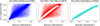 |
Fig. 2 Visualization of the DBSCAN filtering process on the 2014 dataset. Left: The unfiltered relationship between array yield and reference yield, visualized with high point transparency. The overlapping data points reveal a dense, linear trend corresponding to the system's primary operational mode, but it is surrounded by significant noise. Middle: The anomalous data points identified as noise by the DBSCAN algorithm. These outliers, which constitute only around 12% of the total data, are removed from the analysis. Right: The clean, high-density cluster retained after filtering. This cluster, comprising approximately 87% of the original data. Given the consistency, we present the results for a single representative inverter (Inverter 2001). The filtering results for the other two inverters, which show nearly identical patterns, are provided in Appendix A (Figs. A1–A3). |
3.2 Predictive model performance and validation
A separate LGBM model was trained for each of the three inverters using only the DBSCAN-filtered data from the 2014 operational year. The predictive accuracy of each model was first evaluated on a validation set from that same year. The models demonstrated high initial performance, achieving Mean Absolute Percentage Errors (MAPE) of 5.67%, 5.48%, and 5.42% for devices 1001, 1002, and 2001, respectively. This low error confirms the model's ability to accurately represent the system's “as-new” performance baseline.
For the main case study, the training period corresponds to the first calendar year after the end of commissioning, during which the plant had already reached stable operation. Months that still exhibited commissioning artefacts or major interventions were excluded from the training subset. In this sense, the “first year” used for model fitting represents the system's initial steady state rather than an early transient phase, limiting the risk that non-representative behavior biases the long-term degradation estimates.
Following this validation, the fixed model was applied to the chronologically separate, out-of-sample data from all subsequent years (2015–2019) to quantify performance deviation. As shown in Figure 3, the resulting deviation from the 2014 baseline, quantified by the monthly MAPE, is not a simple, steady increase. While there is a subtle upward drift in the baseline deviation, the plot is dominated by several extreme, transient spikes where the MAPE dramatically exceeds 100%. These irregularities, at first glance, could suggest poor model generalization.
However, a detailed investigation, including correspondence with the plant's technical management, revealed that these spikes are not indicative of model failure but are, in fact, successful detections of documented, real-world events. The most extreme anomaly in January 2017, where the monthly MAPE for one inverter reached over 160%, directly corresponds to a period of major site maintenance, during which shutdowns were required to replace approximately half of the plant's underground string cables. Likewise, other major spikes during winter months (e.g., February 2018) were confirmed to coincide with days of heavy snow cover, where actual production was near zero while the model correctly predicted output based on irradiance.
This demonstrates that the LGBM model is performing its function exceptionally well. It serves not only as a stable performance baseline but also as a highly sensitive system-wide event detector. The increasing deviation between the model's predictions and the measured output successfully flags periods of both recoverable losses (snow) and externally-induced downtime (maintenance). This validation is a critical prerequisite for the subsequent analysis, as it confirms the model is providing a meaningful signal, composed of transient anomalies and an underlying degradation trend, which can be decomposed to isolate the true long-term PLR.
Crucially, data from these irregular months are intentionally retained, as the subsequent STL decomposition is designed to robustly separate these transient anomalies from the underlying long-term degradation trend.
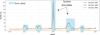 |
Fig. 3 Predictive Model Error (MAPE) Over Time for Three Co-located Inverters. The plot shows the monthly MAPE between measured DC power and the output predicted by the static 2014 baseline model. The growing deviation over time and the sharp spikes are not model failures but are direct indicators of physical system degradation and verified operational anomalies, respectively. This validates the model's use as a sensitive performance baseline. |
3.3 Degradation trend analysis via the performance ratio index (PRI)
To obtain a stable representation of long-term performance evolution, the monthly Performance Ratio Index (PRI) was first computed by normalizing each inverter's measured monthly PR against the expected PR predicted by the baseline LGBM model. Although PRI substantially reduces the influence of irradiance, temperature, and other environmental drivers, the resulting time series still contains seasonal structure and short-term fluctuations that must be separated before the underlying degradation behavior can be evaluated.
The Seasonal–Trend decomposition using LOESS (STL) was therefore applied to the monthly PRI. Figure 4 illustrates this process for Inverter 1001. The observed PRI signal exhibits both scatter and recurrent annual patterns. STL decomposes this signal into three components. The extracted Trend forms a smooth trajectory that reflects the inverter's long-term performance evolution, showing a gradual and continuous decline over the six-year period. The Seasonal component captures the repeating yearly modulation commonly observed in PR-based metrics. Its persistence indicates that the predictive baseline, while accurate, did not fully compensate for complex recurring physical dynamics, thereby necessitating this secondary decomposition step. Finally, the Residual component absorbs short-lived deviations that do not follow a seasonal structure; although brief anomalies are visible, they do not propagate into the Trend component.
The decomposition produces a long-term Trend signal that is considerably less noisy than the raw PRI and no longer influenced by recurring seasonal effects. This Trend is therefore an appropriate input for subsequent analysis. Figure 5 presents the extracted Trend for each inverter at Site A, plotted together with the monthly PRI values. The trends display a broadly consistent downward evolution, though not strictly linear, reflecting the natural variability of multi-year performance behavior. Differences across inverters are most noticeable in the earlier part of the operational life, where small deviations in slope and curvature appear, but these variations diminish as the time series progresses and the long-term dynamics become dominant.
Overall, the PRI–STL pipeline yields a clean and interpretable long-term representation of system behavior that isolates slow performance changes from both seasonal cycles and short-term noise. This extracted Trend forms the foundation for the change-point analysis and phase-resolved degradation quantification presented in the following section.
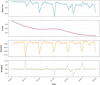 |
Fig. 4 STL Decomposition of the Monthly Performance Ratio Index (PRI) on Inverter 1001. The process separates the noisy original signal (top row) into its constituent parts: a repeating a smooth long-term Trend, Seasonal component, and random Residual noise. This visualization demonstrates how extreme events that cause high MAPE are successfully isolated from the extracted Trend, yielding a clean signal suitable for degradation analysis. |
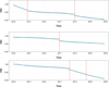 |
Fig. 5 Piecewise linear regression of the extracted PRI degradation trends for the three inverters at Site A. For each inverter, the monthly PRI values (green markers) are shown together with the corresponding piecewise linear best-fit model (blue line). Vertical red dashed lines denote change points detected by the PELT algorithm, partitioning the trend into distinct operational degradation phases. |
3.4 Quantifying non-linear degradation with piecewise regression
The extracted Trend components were subsequently segmented using the PELT changepoint algorithm, allowing for the conversion of the smooth PRI signal into quantitative degradation rates. Because changepoint detection depends on the penalty parameter, several values were tested (0.005, 0.0005, 0.00005, 0.00001) to explore how sensitively the algorithm reacts to fluctuations in the PRI series. For the main case-study results presented here, we focus on an intermediate setting (penalty = 0.0005), which yields a compact number of segments for all three inverters and avoids both a single global fit and very short, difficult-to-interpret segments. The effect of more sensitive penalty choices is examined separately in the following subsection.
Figure 5 shows, for each inverter, the monthly PRI values together with the corresponding piecewise linear fits and the changepoints identified at this baseline penalty. The resulting annual degradation rates for each segment are summarized in Table 1. All estimated slopes are negative, indicating that, once environmental effects are normalized out and the long-term trend is isolated, the PRI trajectories consistently reflect net performance loss rather than spurious improvement.
The phase-resolved rates highlight clear differences in how degradation unfolds for the three inverters. Inverter 1001 displays three phases: an initial, relatively fast decline of −1.422%/year, followed by a much slower intermediate phase of −0.250%/year and a later phase of −0.494%/year. This suggests that early losses are strongest immediately after commissioning and then settle into a more moderate, but still measurable, long-term decline. Inverter 1002 behaves more uniformly, with two phases of −0.165%/year and −0.237%/year; here the changepoint separates two regimes with similar, mild degradation, and the overall trajectory is close to a single shallow linear trend. Inverter 2001 shows a different pattern again: a moderate initial rate of −0.285%/year is followed by a pronounced acceleration to −1.135%/year and then a still elevated final phase of −0.933%/year, indicating that degradation for this device intensifies in the middle of the observation period and remains comparatively high thereafter.
Taken together, these results show that the framework captures inverter-specific degradation histories that would be obscured by a single global PLR value. Early segments mainly reflect commissioning and stabilization behavior, whereas the final segments provide the most relevant indicators for long-term yield expectations: approximately −0.49%/year for inverter 1001, −0.24%/year for inverter 1002, and −0.93%/year for inverter 2001. These values fall within the broad range reported for mono- and poly-Si systems in large fleet studies such as Task 13 PLR report [9], with inverter 2001 representing the upper part of that range but remaining physically plausible for a fielded system.
By combining STL-derived PRI trends, PELT-based segmentation at a clearly specified penalty, and segment-wise linear regression, this step of the framework provides a transparent way to express non-linear ageing as a sequence of phase-specific PLR. The subsequent analysis uses these inverter-level results as the basis for examining penalty sensitivity and for aggregating behavior across the wider fleet.
In many industrial contexts a single aggregate PLR value is still desired for contractual or benchmarking purposes. Within our framework such a scalar can be obtained, if required, by forming an energy- or time-weighted average of the phase-specific slopes reported in Table 1. However, we emphasize that this compression inevitably discards information about operational phases and interventions; throughout this work we therefore interpret the vector of phase-specific PLR as the primary result and use any aggregated PLR only as a secondary, illustrative summary.
We further assessed the robustness of the changepoint detection by systematically varying the PELT penalty parameter and re-analyzing the PRI trend of inverter 1002. As shown in Figure 6, reducing the penalty from the baseline value used in Section 3.4 to 0.00005 and 0.00001 makes the algorithm progressively more sensitive to small fluctuations in the trend. At a penalty of 0.00005 (top panel), several additional changepoints emerge, particularly between 2016 and 2018, where the PRI curve shows gentle curvature. These changepoints subdivide intervals that were previously represented by single, longer segments. When the penalty is reduced further to 0.00001 (bottom panel), the algorithm begins inserting changepoints even in regions where the PRI trend is visually close to linear. This results in a noticeably larger number of very short segments, some lasting only a few months.
This behavior has two practical implications for degradation analysis. First, as the penalty decreases, the segmentation becomes increasingly fine-grained, yielding more phases but also shorter ones. These short segments tend to fit locally well because they cover only limited portions of the time series, yet they typically emerge from subdividing an already coherent downward trend rather than from genuine structural shifts. Consequently, the increase in phase count reflects heightened sensitivity of the algorithm rather than the discovery of new degradation regimes.
Second, as the segmentation becomes increasingly dense, the statistical interpretability of individual phases is reduced. When changepoints occur at short intervals, some resulting segments span only a small number of observations, approaching the scale of normal month-to-month variability in the PRI series. Segments of this length provide limited statistical support for estimating a reliable slope, and their PLR values become sensitive to small local fluctuations rather than reflecting sustained changes in system behavior. In such cases, the segmentation reflects the algorithm's sensitivity rather than distinct, long-duration structural transitions in the degradation trend.
These observations support the use of an intermediate penalty for the main case-study results: it produces a concise and stable set of segments across all three inverters while avoiding the over-fragmentation seen at lower penalties. At the same time, exploring multiple penalty levels provides valuable diagnostic information. Different stakeholders may prioritize different forms of insight—operators focused on early issue detection may prefer a more sensitive segmentation, while those focused on long-term degradation rates may favor fewer, more stable phases. Providing results under multiple penalties therefore helps clarify how segmentation choice influences the granularity of the PLR estimates and allows practitioners to select the configuration best aligned with their analytical objectives.
Importantly, despite the variation in the number and placement of changepoints, the global PRI trajectory remains visually consistent across all tested penalties. The smooth long-term decline from 2014 to 2019 is preserved regardless of segmentation density, indicating that the underlying degradation signal is robust with respect to the penalty parameter.
Annualized degradation rates (PLR, %/year) for each inverter across the piecewise-identified operational phases. Values reflect the slopes of the segment-wise linear regressions fitted to the PRI trends. A dash indicates that no additional segment was detected for that inverter.
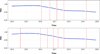 |
Fig. 6 Effect of PELT penalty values on detected changepoints for Inverter 1002. Top: Results using penalty = 0.00005, showing a moderate increase in sensitivity and multiple detected changepoints. Bottom: Results using penalty = 0.00001, where the lower penalty produces a highly sensitive segmentation and a larger number of changepoints. These examples illustrate how penalty selection governs the trade-off between model simplicity and responsiveness to small fluctuations in the PRI trend. |
3.5 Fleet validation and statistical analysis
To evaluate the robustness and scalability of the proposed framework, the full pipeline was applied to eight PV sites covering a wide range of system sizes, data resolutions, and reference-sensor conditions. Figure 7 and Table 2 summarize all segment-wise degradation rates extracted from these sites after STL decomposition, PELT segmentation, and linear regression. Several observations follow.
First, the central tendencies vary substantially across sites, reflecting genuine operating differences rather than a uniform fleet-wide pattern. Sites A and B show medians between −0.39% and −0.44%/year, which lie within the broad range typically reported for crystalline-silicon systems. Other sites exhibit noticeably different behavior: Site C contains several strongly negative phases (median −1.07%/year), while Sites E and F show medians near zero or slightly positive. These deviations are consistent with the suspected reference-sensor issues at these locations. Because DBSCAN suppresses only sparse anomalies, long-duration pyranometer drift or miscalibration can persist into the PRI computation, influencing the extracted degradation rates.
Second, multi-phase degradation behavior is observed across all datasets. The presence of multiple slopes per inverter confirms that non-linear evolution of performance is common among fielded systems, echoing findings from the Task 13 PLR report [9], where early stabilization, mid-life transitions, and system-specific changes appeared frequently. The segment-wise PLR in Figure 7 therefore capture characteristic operational dynamics rather than methodological artifacts.
Extreme positive or negative phase slopes occasionally appear in Figure 7 and Table 2. These values correspond to short-lived operational events—such as seasonal shifts, cleaning, snow cover, or transient mismatches in reference-sensor behavior—rather than to long-term PLR. Because the segmentation isolates local behavior, these short segments appropriately capture transient dynamics without affecting the inference of long-term degradation trends.
Comparison with industry benchmark systems provides additional context for interpreting the fleet-level results. The EURAC and FOSS plants—long-term, well-monitored systems included in the Task 13 PLR report [9] benchmark—have ensemble PLR of −0.85%/year and −0.71%/year, respectively. Because the present framework estimates degradation from segmented PRI trends rather than from a single global regression, numerical differences are expected. The median phase slopes obtained here (EURAC: −1.41%/year; FOSS: −0.09%/year) reflect local, segment-wise behavior and should not be viewed as direct substitutes for the ensemble PLR values. Several factors contribute to these differences: the two systems differ in module technology, climate, and operating histories, and the IEA study itself documents substantial variability across methods for each system, with certain techniques deviating by more than 0.5%/year depending on their filtering and normalization choices. In this context, deviations between PRI-based segmented trends and global PLR estimates are reasonable and consistent with known method-to-method variability. The benchmark comparisons therefore provide external reference ranges confirming that the inferred degradation patterns remain physically plausible.
The segment-wise PLR produced by the framework therefore quantify local degradation behavior within each operational phase rather than providing a direct analogue to the long-term system-wide PLR reported in IEA-PVPS studies.
Finally, despite the site-to-site variability, the framework scales effectively across datasets ranging from 1 to 29 inverters and from 1- to 15-minute sampling intervals without site-specific tuning. This demonstrates that the pipeline can serve as a practical tool for fleet-level screening, provided that the underlying irradiance data are reliable. The fleet analysis therefore reinforces both the strengths of the approach—its ability to isolate multi-phase degradation—and its main limitation, namely sensitivity to the accuracy and stability of reference sensors.
A known limitation of the present implementation is that long-lasting drifts or step changes in reference sensor behavior are not explicitly corrected for within the DBSCAN–LGBM–PRI pipeline itself. DBSCAN efficiently removes short-lived outliers and obvious artefacts, but a slowly degrading pyranometer, for instance, would manifest as an apparent change in the irradiance–power relationship and could be partially absorbed into the degradation signal. In our case-study fleet we mitigated this risk qualitatively by cross-checking against redundant telemetry and maintenance logs, and by interpreting unusually steep phase slopes in the context of known sensor issues; a fully automated treatment of sustained sensor failure will be an important focus of future work.
From a statistical perspective, the fleet-level distributions in Figure 7 and the high coefficients of determination reported in Table 2 indicate that, within each detected phase, the linear degradation assumption provides an excellent fit to the STL-derived Trend. While we do not report formal confidence intervals or hypothesis tests in this paper, the narrow interquartile ranges of the fleet PLR distributions, together with the consistency of our central tendencies with independently reported benchmark plants such as EURAC and FOSS, suggest that the observed variation in PLR values (for example the −0.78 to −0.20%/year range reported for the main case study) reflects genuine site-to-site and phase-to-phase differences rather than being dominated by random noise alone. A dedicated uncertainty analysis based on bootstrapping or Bayesian regression is planned as a natural extension of this work.
Summary statistics of phase-specific degradation rates across eight PV sites. The table reports descriptive statistics for the segment-wise degradation rates (%/year) underlying the boxplots in Figure 7. For each site, the number of inverters analyzed, and the total analysis period are listed, followed by the minimum, lower quartile (Q1), median, upper quartile (Q3), and maximum phase degradation rates derived from the piecewise linear regression of PRI trends.
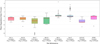 |
Fig. 7 Distribution of phase-specific degradation rates obtained from the proposed framework across eight PV sites. Each boxplot summarizes the slopes of all piecewise linear segments identified for all inverters at a given site, illustrating the variability in degradation behavior across phases and system locations. Site labels include the number of inverters analyzed and the average number of detected phases per inverter. |
4 Discussion
This work proposes a unified degradation-analysis framework that integrates unsupervised filtering, machine-learning-based normalization, and change-point-aware trend modeling. Applied first to three co-located inverters and then to a broader fleet spanning eight sites, the framework demonstrates three strengths: its ability to isolate long-term degradation from environmental variability, its capacity to reveal non-linear multi-phase behavior, and its robustness across systems with different sizes, conditions, and data qualities.
A core contribution is the use of DBSCAN for adaptive noise filtering. Unlike static rule-based thresholds, the density-driven filter retains approximately 80% of the operational data while reliably excluding sparse anomalies. This high-retention approach provides a stronger statistical foundation for the predictive model and reduces the risk of filter-induced bias documented in prior PLR studies. The resulting dataset preserves the full range of environmental conditions and supports stable estimation of the expected DC power.
The second contribution is the use of a fixed early-life LGBM baseline to establish a weather-normalized Performance Ratio Index (PRI). The PRI compresses high-resolution operational data into a monthly, environmentally corrected performance signal that is smoother and more interpretable than raw PR. The reviewer-highlighted concern regarding early-year instability is addressed through the segmentation stage: any non-representative early-life behavior forms its own distinct phase and therefore does not influence the long-term degradation rate. In the case study, although one inverter shows atypical early-year behavior, the changepoint detection successfully isolates this interval, and the later phases converge to stable long-term degradation trends.
The third contribution is the explicit characterization of non-linear behavior through STL decomposition and PELT segmentation. This process identifies structural breaks and yields phase-specific degradation rates. The results at the baseline penalty reveal clear multi-phase dynamics that are consistent with observations from long-term PV fleet studies. The sensitivity analysis further shows how penalty selection governs the balance between interpretability and detection granularity: lower penalties introduce additional short segments, but these typically refine rather than fundamentally alter the dominant downward trajectory. This confirms that the long-term signal is robust, even though the degree of segmentation is user dependent.
Fleet-level validation across eight sites underscores both the strengths and the limitations of the approach. On the positive side, most commercial sites exhibit median phase-specific slopes within the broad range expected for crystalline-silicon systems. The EURAC and FOSS benchmark datasets also show phase-specific trends that are physically plausible, even though their segment-wise medians do not numerically coincide with the ensemble PLR reported in the IEA-PVPS Task 13 study. This is expected: the benchmarks are defined using global system-wide regression, whereas the present framework produces local segment-wise rates, and the IEA study itself shows substantial method-dependent variability across filtering and normalization choices. Thus, the benchmark comparisons serve as contextual references rather than one-to-one validation targets.
The main limitation revealed by the fleet analysis concerns the reliance on high-quality irradiance measurements [4]. Persistent pyranometer drift, long-duration sensor bias, or inconsistent inverter-sensor mapping can propagate through the PRI calculation [4] and broaden the distribution of extracted slopes, as observed for Sites E and F. Multiple pyranometers per site introduce further spread when all pairings are evaluated. These findings suggest that future extensions of the framework should incorporate sensor-quality diagnostics or automated sensor-selection logic.
When considered in light of these results, the framework bridges two scales of PV performance analysis: detailed inverter-level diagnosis and fleet-wide statistical assessment. It provides a transparent, modular structure for isolating degradation signals, quantifying multi-phase behavior, and evaluating sensitivity to segmentation granularity. Although further validation across more technologies and climates is warranted, the results demonstrate that the method produces physically interpretable trends consistent with established knowledge while offering new flexibility for practical operational analytics.
5 Conclusion
This study introduces a scalable and interpretable framework for quantifying photovoltaic performance loss rates by combining adaptive data filtering, machine-learning-based normalization, and change-point-aware trend analysis. Applied to six years of high-resolution data from three co-located inverters, the methodology successfully isolates long-term degradation dynamics from short-term operational anomalies and seasonal variability. The resulting phase-resolved degradation rates provide a more informative description of system behavior than a single global PLR.
Extending the framework to a diverse fleet of eight sites demonstrates its robustness across varied operating conditions, measurement resolutions, and inverter populations. The extracted degradation rates fall within physically plausible ranges and are consistent with patterns reported in large international studies [2], while the segment-wise representation reveals additional structure relevant for operational monitoring and asset evaluation. The analysis also highlights that reference-sensor quality remains a central determinant of accuracy, motivating future work on automated sensor assessment and improved irradiance normalization.
Overall, the framework offers a practical tool for both system-level diagnosis and fleet-wide benchmarking, supporting more informed decision-making in long-term PV asset management. Future research will focus on integrating sensor-quality metrics, comparing directly with established PLR methods such as YoY and RDTools, and expanding validation across additional technologies and climates.
Glossary
Artificial Neural Networks (ANN): A machine learning model inspired by biological neural networks, capable of learning complex, non-linear relationships from large datasets, used in this study to model dependencies between environmental inputs and PV system output.
Array Yield (Ya): The PV array's DC energy output per unit of installed DC nameplate power at STC (Ya = EDC / P0; unit: kWh/kWp).
Change Point Detection: A statistical method to identify points in a time series where the underlying data properties (e.g., mean, variance) shift, used in this work to detect transitions in degradation phases via the PELT algorithm.
DBSCAN (Density-Based Spatial Clustering of Applications with Noise): An unsupervised clustering algorithm that groups closely packed data points and identifies outliers in low-density regions, used for adaptive filtering of PV operational data to remove anomalies while preserving around 80% of valid data.
DC Power: The direct current power output from the PV array before conversion to alternating current by the inverter, measured in kilowatts (kW) and used as a primary variable for performance analysis.
Degradation Signal: The component of the PV system's performance data that reflects long-term performance decline, isolated in the manuscript through the Performance Ratio Index (PRI) and STL decomposition.
Inverter: A device that converts direct current (DC) power from PV modules into alternating current (AC) for grid integration. In this work, the term collectively refers to the devices across the entire analyzed fleet of 84 inverters at 8 distinct locations , with a detailed comparative degradation analysis focusing on three co-located inverters (Inverter 1001, 1002, and 2001) at Site A.
LGBM (Light Gradient Boosting Machine): An ensemble decision-tree-based machine learning model used to predict expected DC power output, selected for its accuracy and efficiency in establishing a weather-normalized performance baseline.
MAPE (Mean Absolute Percentage Error): A metric used to evaluate the predictive accuracy of the LGBM model, calculated as the average absolute percentage difference between actual and predicted DC power values, expressed as a percentage.
O&M (Operations and Maintenance): Activities to ensure the optimal performance and longevity of PV systems, including monitoring, cleaning, and repairs, critical for mitigating reversible performance losses.
PELT (Pruned Exact Linear Time): An algorithm for detecting change points in time series data by minimizing a penalized cost function, used to identify structural breaks in the degradation trend with a modified BIC penalty.
Performance Loss Rate (PLR): The annualized rate at which a PV system's performance declines, expressed as a percentage per year, quantified in this study using piecewise linear regression on the STL trend.
Performance Ratio Index (PRI): A derived metric formed by the ratio of actual to predicted Performance Ratio (PRactual/PRpredicted), used to quantify intrinsic performance changes while accounting for environmental variations.
Piecewise Linear Regression: A method to model non-linear trends by fitting separate linear segments to different time periods, applied to quantify PLR in distinct degradation phases after PELT change point detection.
POA Irradiance (Plane of Array Irradiance): The solar irradiance received by the PV array's surface, measured in W/m2, used as a key input for the LGBM predictive model.
Reference Yield (Yr): The equivalent number of hours at the reference irradiance of 1 kW/m2 that would deliver the same plane-of-array irradiance measured over the period; numerically, Yr = Hpoa / Gref with Gref = 1 kW/m2, expressed in hours (kWh/kW).
STL (Seasonal-Trend Decomposition using LOESS): A time-series decomposition method that separates data into trend, seasonal, and residual components, used to isolate the long-term degradation trend from the PRI time series.
Funding
This research did not receive any direct financial support. The authors acknowledge the institutional support and data access provided by saferay holding GmbH and Wattmanufactur GmbH & Co. KG.
Conflicts of interest
The authors declare that they have no conflict of interest.
Data availability statement
The core commercial datasets (Site A and Validation Fleet Sites B–F) analyzed in this study were provided by industrial partners and are not publicly available due to commercial confidentiality agreements. However, the methodology and code are described in sufficient detail to allow replication on similar datasets. Importantly, the analysis was benchmarked using authoritative public datasets: the EURAC Research and FOSS Research Centre PV systems, which are publicly available for reference in the IEA PVPS Task 13 PLR report dataset compilation.
Author contribution statement
Kak-Pong Cheung: Conceptualization, Methodology, Software, Formal analysis, Investigation, Writing – Original Draft.
Stephanie Malik: Supervision, Writing – Review & Editing
David Daßler: Supervision, Writing – Review & Editing.
Carsten Hennig: Conceptualization, Project Administration, Data Provisioning.
Hauke Nissen: Conceptualization, Project Administration, Data Provisioning.
Patrick Hennig: Supervision, Project Administration, Writing – Review & Editing.
Use of AI in manuscript preparation
The authors utilized the generative AI language model, ChatGPT (model 4o), to assist in polishing the language and improving the readability of this manuscript. All intellectual content, including research concepts, methodology, and analysis, is the original work of the authors.
References
- S. Lindig, J. Ascencio-Vásquez, J. Leloux, D. Moser, A. Reinders, Performance analysis and degradation of a large fleet of PV systems, IEEE J. Photovolt. 11, 1312 (2021). https://doi.org/10.1109/JPHOTOV.2021.3093049 [CrossRef] [Google Scholar]
- D.C. Jordan, K. Anderson, K. Perry, M. Muller, M. Deceglie, R. White, C. Deline, Photovoltaic fleet degradation insights, Prog. Photovolt. Res. Appl. 30, 1166 (2022). https://doi.org/10.1002/pip.3566 [CrossRef] [Google Scholar]
- A. Louwen, S. Lindig, G. Chowdhury, D. Moser, Climate- and technology-dependent performance loss rates in a large commercial photovoltaic monitoring dataset, Sol. RRL 8, 2300653 (2024). https://doi.org/10.1002/solr.202300653 [Google Scholar]
- S. Lindig, M. Herz, J. Ascencio-Vásquez, M. Theristis, B. Herteleer, J. Deckx, K. Anderson, Review of technical photovoltaic key performance indicators and the importance of data quality routines, Sol. RRL 8, 2400634 (2024). https://doi.org/10.1002/solr.202400634 [Google Scholar]
- IEA, Guidelines for operation and maintenance of photovoltaic power plants in different climates (IEA-PVPS, Paris, 2022) [Google Scholar]
- D.C. Jordan, S.R. Kurtz, Photovoltaic degradation rates - an analytical review, Prog. Photovolt. Res. Appl. 21, 12 (2013). https://doi.org/10.1002/pip.1182 [Google Scholar]
- P. Gupta, R. Singh, PV power forecasting based on data-driven models: a review, Int. J. Sustain. Eng. 14, 1733 (2021). https://doi.org/10.1080/19397038.2021.1986590 [Google Scholar]
- M.J. Mayer, G. Gróf, Extensive comparison of physical models for photovoltaic power forecasting, Appl. Energy 283, 116239 (2021). https://doi.org/10.1016/j.apenergy.2020.116239 [Google Scholar]
- IEA, Assessment of performance loss rate of PV power systems (IEA-PVPS, Paris, 2021) [Google Scholar]
- IEA, The use of advanced algorithms in PV failure monitoring (IEA-PVPS, Paris, 2021) [Google Scholar]
- K. Anderson, C. Hansen, W. Holmgren, A. Jensen, M. Mikofski, A. Driesse, Pvlib Python: 2023 project update, J. Open Source Softw. 8, 5994 (2023). https://doi.org/10.21105/joss.05994 [CrossRef] [Google Scholar]
- M. Ester, H.-P. Kriegel, J. Sander, X. Xu, A density-based algorithm for discovering clusters in large spatial databases with noise, in Proceedings of the Second International Conference on Knowledge Discovery and Data Mining (KDD-96), E. Simoudis, J. Han, U.M. Fayyad (Eds.), (AAAI Press, Portland, 1996), pp. 226–231 [Google Scholar]
- C. Lartey, J. Liu, R. K. Asamoah, C. Greet, M. Zanin, W. Skinner, Effective outlier detection for ensuring data quality in flotation data modelling using machine learning (ML) algorithms, Minerals 14, 925 (2024). https://doi.org/10.3390/min14090925 [Google Scholar]
- G. Ke, Q. Meng, T. Finley, T. Wang, W. Chen, W. Ma, Q. Ye, T. Y. Liu, LightGBM: a highly efficient gradient boosting decision tree, in Advances in Neural Information Processing Systems 30 (NeurIPS 2017), I. Guyon, U. V. Luxburg, S. Bengio, H. Wallach, R. Fergus, S. Vishwanathan, R. Garnett (Eds.),(Curran Associates, Red Hook, NY, 2017), p. 3146. https://proceedings.neurips.cc/paper_files/paper/2017/file/6449f44a102fde848669bdd9eb6b76fa-Paper.pdf [Google Scholar]
- G. Guerra, P. Mercade-Ruiz, G. Anamiati, L. Landberg, Long-term PV system modelling and degradation using neural networks, EPJ Photovolt. 14, 30 (2023). https://doi.org/10.1051/epjpv/2023018 [CrossRef] [EDP Sciences] [Google Scholar]
- M.G. Deceglie, K. Anderson, A. Shinn, N. Ambarish, M. Mikofski, M. Springer, J. Yan, K. Perry, S. Villamar, W. Vining, G.M. Kimball, D. Ruth, N. Moyer, Q. Nguyen, D. Jordan, M. Muller, C. Deline, RdTools [Computer software], Zenodo (2018). https://doi.org/10.5281/zenodo.1210316 [Google Scholar]
- D. Jordan, C. Deline, S. Kurtz, G. Kimball, M. Anderson, Robust PV degradation methodology and application, IEEE J. Photovolt. 8, 525 (2018). https://doi.org/10.1109/JPHOTOV.2017.2779779 [CrossRef] [Google Scholar]
- R.B. Cleveland, W.S. Cleveland, J.E. McRae, I. Terpenning, STL: a seasonal-trend decomposition procedure based on loess, J. Off. Stat. 6, 3 (1990). https://www.math.unm.edu/lil/Stat581/STL.pdf [Google Scholar]
- R. Killick, P. Fearnhead, I.A. Eckley, Optimal detection of changepoints with a linear computational cost, J. Am. Stat. Assoc. 107, 1590 (2012). https://doi.org/10.1080/01621459.2012.737745 [CrossRef] [Google Scholar]
- C. Truong, L. Oudre, N. Vayatis, Selective review of offline change point detection methods, Signal Process. 167, 107299 (2020). https://doi.org/10.1016/j.sigpro.2019.107299 [CrossRef] [Google Scholar]
- Z. Gao, X. Xiao, Y.-P. Fang, J. Rao, H. Mo, A selective review on information criteria in multiple change point detection, Entropy 26, 50 (2024). https://doi.org/10.3390/e26010050 [Google Scholar]
- M. Lavielle, Using penalized contrasts for the change-point problem, Signal Process. 85, 1501 (2005). https://doi.org/10.1016/j.sigpro.2005.01.012 [Google Scholar]
- K. Haynes, I.A. Eckley, P. Fearnhead, Computationally efficient changepoint detection for a range of penalties, J. Comput. Graph. Stat. 26, 134 (2017). https://doi.org/10.1080/10618600.2015.1116445 [CrossRef] [Google Scholar]
Cite this article as: Kak-Pong Cheung, Stephanie Malik, David Daßler, Carsten Hennig, Hauke Nissen, Patrick Hennig, A comprehensive framework for accurate estimation of performance loss rates in large photovoltaic systems using machine learning, EPJ Photovoltaics 17, 8 (2026), https://doi.org/10.1051/epjpv/2026001
Appendix
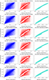 |
Fig. A1 DBSCAN filtering results for Device 1001 from 2014 to 2019. The stability of the retained 'Non-Noise' cluster (right column) across all years demonstrates the effectiveness of the method. |
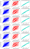 |
Fig. A2 DBSCAN filtering results for Device 1002 from 2014 to 2019. The results show a highly consistent filtering performance, mirroring the patterns observed for the other devices. |
 |
Fig. A3 DBSCAN filtering results for Device 2001 from 2014 to 2019. The visual evidence confirms that the DBSCAN method reliably isolates the core operational data, providing a robust input for the subsequent modeling stages. |
All Tables
Annualized degradation rates (PLR, %/year) for each inverter across the piecewise-identified operational phases. Values reflect the slopes of the segment-wise linear regressions fitted to the PRI trends. A dash indicates that no additional segment was detected for that inverter.
Summary statistics of phase-specific degradation rates across eight PV sites. The table reports descriptive statistics for the segment-wise degradation rates (%/year) underlying the boxplots in Figure 7. For each site, the number of inverters analyzed, and the total analysis period are listed, followed by the minimum, lower quartile (Q1), median, upper quartile (Q3), and maximum phase degradation rates derived from the piecewise linear regression of PRI trends.
All Figures
|
Fig. 1 Overview of the proposed degradation analysis framework. |
| In the text | |
|
Fig. 2 Visualization of the DBSCAN filtering process on the 2014 dataset. Left: The unfiltered relationship between array yield and reference yield, visualized with high point transparency. The overlapping data points reveal a dense, linear trend corresponding to the system's primary operational mode, but it is surrounded by significant noise. Middle: The anomalous data points identified as noise by the DBSCAN algorithm. These outliers, which constitute only around 12% of the total data, are removed from the analysis. Right: The clean, high-density cluster retained after filtering. This cluster, comprising approximately 87% of the original data. Given the consistency, we present the results for a single representative inverter (Inverter 2001). The filtering results for the other two inverters, which show nearly identical patterns, are provided in Appendix A (Figs. A1–A3). |
| In the text | |
|
Fig. 3 Predictive Model Error (MAPE) Over Time for Three Co-located Inverters. The plot shows the monthly MAPE between measured DC power and the output predicted by the static 2014 baseline model. The growing deviation over time and the sharp spikes are not model failures but are direct indicators of physical system degradation and verified operational anomalies, respectively. This validates the model's use as a sensitive performance baseline. |
| In the text | |
|
Fig. 4 STL Decomposition of the Monthly Performance Ratio Index (PRI) on Inverter 1001. The process separates the noisy original signal (top row) into its constituent parts: a repeating a smooth long-term Trend, Seasonal component, and random Residual noise. This visualization demonstrates how extreme events that cause high MAPE are successfully isolated from the extracted Trend, yielding a clean signal suitable for degradation analysis. |
| In the text | |
|
Fig. 5 Piecewise linear regression of the extracted PRI degradation trends for the three inverters at Site A. For each inverter, the monthly PRI values (green markers) are shown together with the corresponding piecewise linear best-fit model (blue line). Vertical red dashed lines denote change points detected by the PELT algorithm, partitioning the trend into distinct operational degradation phases. |
| In the text | |
|
Fig. 6 Effect of PELT penalty values on detected changepoints for Inverter 1002. Top: Results using penalty = 0.00005, showing a moderate increase in sensitivity and multiple detected changepoints. Bottom: Results using penalty = 0.00001, where the lower penalty produces a highly sensitive segmentation and a larger number of changepoints. These examples illustrate how penalty selection governs the trade-off between model simplicity and responsiveness to small fluctuations in the PRI trend. |
| In the text | |
|
Fig. 7 Distribution of phase-specific degradation rates obtained from the proposed framework across eight PV sites. Each boxplot summarizes the slopes of all piecewise linear segments identified for all inverters at a given site, illustrating the variability in degradation behavior across phases and system locations. Site labels include the number of inverters analyzed and the average number of detected phases per inverter. |
| In the text | |
|
Fig. A1 DBSCAN filtering results for Device 1001 from 2014 to 2019. The stability of the retained 'Non-Noise' cluster (right column) across all years demonstrates the effectiveness of the method. |
| In the text | |
|
Fig. A2 DBSCAN filtering results for Device 1002 from 2014 to 2019. The results show a highly consistent filtering performance, mirroring the patterns observed for the other devices. |
| In the text | |
|
Fig. A3 DBSCAN filtering results for Device 2001 from 2014 to 2019. The visual evidence confirms that the DBSCAN method reliably isolates the core operational data, providing a robust input for the subsequent modeling stages. |
| In the text | |
Current usage metrics show cumulative count of Article Views (full-text article views including HTML views, PDF and ePub downloads, according to the available data) and Abstracts Views on Vision4Press platform.
Data correspond to usage on the plateform after 2015. The current usage metrics is available 48-96 hours after online publication and is updated daily on week days.
Initial download of the metrics may take a while.