| Issue |
EPJ Photovolt.
Volume 16, 2025
Special Issue on ‘EU PVSEC 2024: State of the Art and Developments in Photovoltaics’, edited by Robert Kenny and Gabriele Eder
|
|
|---|---|---|
| Article Number | 25 | |
| Number of page(s) | 20 | |
| DOI | https://doi.org/10.1051/epjpv/2025011 | |
| Published online | 27 May 2025 | |
https://doi.org/10.1051/epjpv/2025011
Original Article
Analysis of fault detection and defect categorization in photovoltaic inverters for enhanced reliability and efficiency in large-scale solar energy systems
1
Fraunhofer IMWS, Fraunhofer Institute for Microstructure of Materials and Systems, Walter-Hülse-Str. 1, Halle
06120, Germany
2
DiSUN, Deutsche Solarservice GmbH, Mielestr. 2, Werder 14542, Germany
3
DENKweit GmbH, Blücherstr. 26, Halle 06120, Germany
4
Saferay holding GmbH, Rosenthaler Str. 34/35, Berlin 10178, Germany
5
Leipziger Energiegesellschaft mbH & Co. KG, Burgstraße 1, Leipzig 504109, Germany
* e-mail: This email address is being protected from spambots. You need JavaScript enabled to view it.
Received:
30
September
2024
Accepted:
27
March
2025
Published online: 27 May 2025
Abstract
This study presents a systematic approach for examining the performance and vulnerability of large-scale, grid-connected PV systems in relation to inverter faults − particularly those linked to insulated-gate bipolar transistor (IGBT) component. The focus is on an interdisciplinary approach, utilising methodologies from materials science, data analysis, statistics, and machine learning to investigate defect mechanisms, identify recurring issues, and analyse their impacts for a system portfolio of 64 MWp. A root cause analysis identified the failure pattern through material diagnostics of several power modules from inverters previously installed in the field. Prolonged exposure to high temperatures led to the degradation of the IGBT semiconductors, resulting in a breakthrough due to the short-term release of excessive heat. In parallel, an impact analysis was carried out based on historical monitoring data, that identified a faulty control behaviour of the inverter during curtailment. Due to the sharp increase in curtailment occurrences, a correlation of this observation was noted across nearly the entire portfolio. Finally, the study explored whether this randomly observed fault pattern that led to the inverter failure could have been detected in the data without prior knowledge of it. To achieve this, a method combining an artificial neural network and density-based clustering was proposed to automatically detect this recurring and propagating error pattern. This process was carried out in three steps: predicting the normal behaviour of the inverter, distinguishing between normal behaviour and anomalous behaviour, and differentiating the anomalous behaviour. The fault patterns were clearly assigned to four clusters. By introducing a scalable, data-driven fault diagnostics method, this study highlights how advanced materials science and data analytics can improve early fault detection and maintenance in PV portfolio monitoring, while also providing a deeper understanding of defect mechanisms. These combined approaches ultimately enhance inverter reliability and operational efficiency.
Key words: Inverter failure / material diagnostics / data analysis / fault detection / curtailment / machine learning
© S. Malik et al., Published by EDP Sciences, 2025
 This is an Open Access article distributed under the terms of the Creative Commons Attribution License (https://creativecommons.org/licenses/by/4.0), which permits unrestricted use, distribution, and reproduction in any medium, provided the original work is properly cited.
1 Introduction
The optimal integration of photovoltaics (PV) is crucial for reducing greenhouse gas emissions and ensuring a sustainable energy supply. Inverters are key components for connecting solar modules to the public power grid by converting direct current (DC) into grid-compatible alternating current (AC). Inverters are also responsible for monitoring, communication as well as the regulation of the power output through curtailment or maximum power point optimisation.
Failures or malfunctions of inverters can lead to partial or complete shutdowns of PV systems, resulting in substantial financial losses for operators and investors, combined with increasing maintenance and operating costs. To ensure that PV systems can be operated continuously, it is necessary to understand the defect mechanisms of inverter failures and to reduce their extent and impact during operation. Studies [1–3] report that around 50% of failures in PV systems are related to inverters. Furthermore, the high number of operation and maintenance (O&M) tickets (43–70%) are caused by inverter defects, requiring a considerable amount of time and personnel resources [1]. Inverters are generally considered to have a shorter operational lifetime compared to PV modules [4]. Nowadays, while PV modules are designed to last for over 30 years, inverters may need calibration, replacement, or repair every 10 to 15 years. They are subjected to various internal and external stresses, such as thermal cycling, grid influences, as well as environmental conditions, including dust and humidity. Prolonged operation under these conditions can lead to failures and performance degradation. The most common types of inverter failures are overheating, material fatigue of components, control and communication failures, grid disturbance, and electrical overload [5,6].
Thermal cycling is one of the primary contributors to material ageing in power electronic devices. As inverters operate, power transistors such as IGBT frequently switch on and off, generating heat. The cycling heating can cause thermal expansion and contraction in the semiconductor material and surrounding packaging. Over time, the repeated thermal cycling can lead to thermal fatigue, where the materials, such as solder, wire bonds, and encapsulating materials begin to deform, dissolve, degrade, or crack. These microscopic changes gradually enhance during continuing operating, potentially leading increased electrical resistances, reduced thermal conductivity, and eventually component failure. In addition, thermal issues can be accelerated by harsh environmental conditions or insufficient cooling [6,7].
The scale of PV deployment continues to grow, with billions of systems installed globally and an increasing number of large-scale solar farms [8]. Although O&M is supporting operations, in general, the demand for quality and efficiency of these services is struggling to keep pace with this rapid expansion. Particularly in large-scale PV systems, where dozens or hundreds of inverters operate simultaneously, the risks posed by inverter failures are magnified. Under such conditions, an efficient O&M service is critical to mitigate technical risks and to achieve optimal energy output [9].
O&M services can consist of several actions: preventive maintenance, such as monitoring and regular inspections, corrective maintenance, for repairing and correcting critical problems, and predictive maintenance, deriving maintenance strategies based on historical operation data [10]. However, managing O&M in large-scale systems presents unique challenges due to the vast number of components, geographical and climatic deviations, and complex variety of system portfolios [11,12]. Effective O&M of large system portfolios requires early detection of inverter deteriorations and an advanced understanding of their failure mechanisms to enable predictive and preventive maintenance. The combination of preventive and predictive maintenance attempts to predict and prevent recurring patterns based on historical findings. These strategies minimise unplanned downtime and reduce the need for costly, reactive repairs.
In contrast to traditional methods that rely predominantly on threshold-based monitoring and reactive maintenance, our approach introduces a multi-layered diagnostic framework that integrates advanced time series processing, machine learning and materials science. Previous studies have demonstrated the value of machine learning methods for fault detection and performance evaluation in PV systems. Dassler et al. [13] explored the applicability of artificial neural networks (ANN) to assess PV system yield, showcasing how clustering techniques can improve fault identification. Their later work [14] refined ANN training strategies to enhance fault detection accuracy. Rupakula et al. [15] proposed an automatic fault classification model using machine learning algorithms, demonstrating its effectiveness in identifying faults such as snow cover, degradation, and outages. Dassler et al. [16] further examined the role of data availability and quality in defect detection, highlighting the importance of reliable data preprocessing and monitoring strategies. While these studies have made significant progress, challenges remain in terms of scalability and integrating physical failure mechanisms into data-driven models. Our study builds upon this foundation by incorporating material diagnostics, providing a more comprehensive framework for understanding inverter failures.
While recent studies have demonstrated the potential of data-driven methods for early fault detection, root cause analysis, and recommendations of remedial actions are needed. Additionally, several gaps remain within inverter diagnostics, particularly for large-scale plants, including the scalability of detection systems, pattern recognition, and stresses caused by environmental impact factors. Our methodology addresses these gaps by combining inverter monitoring data with laboratory-based material diagnostics, enabling not only the identification of subtle defect patterns but also a detailed characterisation of underlying failure mechanisms in inverter components. This integrated approach enhances predictive accuracy for operation and performance, reduces mean time to detect (MTTD) and mean time to repair (MTTR), and offers a scalable solution tailored to the complexities of large PV portfolios. Such improvements represent a significant advancement over existing techniques and contribute novel insights to the field of inverter diagnostics and reliability.
This study examines the performance and vulnerability of large-scale, grid-connected PV systems in relation to inverter faults attributed to the IGBT component. The work presents an interdisciplinary approach, utilising methodologies from materials science, data analysis, and statistics to investigate causes and effects of these malfunctions to understand defect mechanisms, identify repeating problems, and analyse their impacts in portfolios. It will consider the topic of severity of inverter failures assigned to the IGBT component from two sides: Root Cause Analysis and Impact Analysis. The former explores failure causes through material diagnostics, drawing conclusions on potential failure mechanisms based on error messages and material fatigue of defective inverter components from the field. The latter employs pattern recognition in monitoring data − from the defective devices examined in the laboratory − to automatically detect recurring and propagating error patterns, as well as to determine the associated operational risks.
2 Material and methods
2.1 Data source and system portfolio
This study is grounded in extensive datasets, encompassing monitoring data from large PV systems, with a total capacity of 64.4 MWp and spanning multiple years of operation. These datasets, which include high temporal resolution information on inverter operation, establish a robust foundation for analysis. The initial step involved a rigorous assessment of data quality, employing stringent criteria to ensure the plausibility, completeness, and consistency of the available data.
The investigation focused on 102 subsystems, each equipped with a central inverter of the same type in the 500 to 700 kWp range, distributed across three large PV parks, monitored over a period of twelve years (from 2012–2023) in moderate climate conditions. The three PV parks are installed near each other in Germany. The data foundation (see Tab. 1) comprised inverter measurement data and status information, as well as irradiance measured by pyranometers in the module plane with a high temporal resolution of one minute. The systems are equipped with crystalline modules. Ambient temperature data were downloaded from the national weather service [17], specifically for a nearby regional city.
It was assumed that malfunctions or defects in PV systems slightly change the general structure of the operational data, from minor to severe deviations. Possible yield losses do not have to occur immediately but may arise later. Faults without these changes in operating data are unlikely to contribute to yield losses in the near future. Consequently, inverter faults or error conditions also cause deviations that can be found in operating data. With the help of information and protocols from the operators, error messages from the monitoring, and time series evaluation methods, the inverter data were examined for abnormal behaviour.
Overview of the available parameters per inverter (area: inverter) and per system (system status and environment). The values are available at a 1-minute time resolution.
2.2 Root cause analysis
For this study, several power modules from field inverters were provided, including—both failed and functional—devices, to determine the degree of damage and the actual cause of failure. To proceed as sensitively as possible and to minimise the risk of the damage pattern being impaired by preparation steps, non-destructive characterisation methods such as X-ray inspection and scanning acoustic microscopy (SAM) are generally used as a first step. These can already provide initial insights into the level of damage and help to localise the origin. The next step was to expose the damaged area by opening the housing and removing the encapsulation. In case of overload-related failures of power semiconductors, thermal energy is released to such an extent that often the level of damage no longer allows a specific detailed analysis of the failure root cause. Since further analysis appeared feasible and potentially insightful, low-artefact preparation methods and subsequent microstructure analyses were applied. The aim of the investigations was to obtain information on material interactions that have taken place (intrinsic or extrinsic), as well as thermal or mechanical loads that have occurred, the associated degradation mechanisms, and causes of failure. Classical metallographic methods such as grinding and polishing using abrasive papers, cloths, and suspensions along with ion beam techniques were typically used for cross-sectioning. Ion beam based preparation methods are limited in terms of the maximum possible cross-section dimension but minimise the risk of artefacts being introduced. The range of analytical procedures and methods is complex and extends from imaging procedures such as light microscopy and scanning electron microscopy (SEM), through structural analysis methods to element identification and mechanical property determination.
2.3 Impact analysis
This part of the study focuses on the monitoring data and investigates whether a randomly observed fault pattern, which led to the inverter failure, could also have been detected in the data using machine learning. Following this section, the data preparation and two machine learning methods which, in combination, demonstrate how regular and non-regular behaviour can be distinguished and further differentiated, are described. In this context, regular stands for real system behaviour, which corresponds to the majority of the data without being under the influence by abnormalities or existing faulty states. Non-regular stands for outliers that are further away from the regular state.
2.3.1 Modelling of regular system operating behaviour with artificial neuronal networks
Regular system operating behaviour in this context refers to the expected DC and AC power that should be available under the existing ambient conditions but does not include any erroneous states or derating. The methodology used here to predict a regular system operating behaviour of one inverter, in terms of DC and AC power, is based on an artificial neural network, specifically, a feedforward network or multilayer perceptron (for simplicity, in the following term as ANN). The result of the ANN should serve as a reference value for the subsequent cluster step. The ANN model used in this study is based on preliminary work described in detail in [13,14], and [16].
Reframed for flow and scientific objectivity: ANNs can model complex non-linear relationships in data, they can handle large datasets, making them suitable for big data applications, ANNs can be resilient to noise in the input data, maintaining performance despite variations. A feedforward ANN is composed of different layers, which themselves consist of different numbers of nodes (so-called neurons). Each individual neuron is completely connected with all neurons of the adjacent layers. The connections between the neurons (so-called weights) take over the function of storing the structural dependency between given input and output information. Furthermore, an activation function within a neuron transforms the incoming signal into the final output signal. The weights of an untrained ANN are predefined systematically or randomly. To adapt the weights to the data, a training process must be carried out using an initial dataset (training data). During the training, the weights are iteratively adjusted by an optimisation procedure until a termination criterion is reached.
The training process can be controlled by a variety of hyperparameters, which influence how the model learns by tuning weights during the training process. Proper hyperparameter selection is crucial to avoid under- or overfitting of the model and improves the learning process. The meaning of the hyperparameters used for modelling is briefly described below and listed in Table 2:
Batch sise: Represents a small number of training samples taken at a time during training.
Activation function: Determines the scope of the final output of each neuron in the network. The ReLU (Rectified Linear Unit) activation function was chosen due to its computational efficiency.
Optimiser: An algorithm for adapting the weights based on gradient information per iteration step. In this study ADAM (Adaptive Moment Estimation) optimiser was used due to its efficiency with large datasets, robustness to noise and its adaptive learning rates.
Loss function: Measures the quantity of prediction errors raised in the neural network during training and drives the weight update process. In this context, the Huber Loss function was used, which is particularly useful in applications where outliers are present and stable learning processes are required. The Huber Loss function combines the benefits of Mean Squared Error (MSE) and Mean Absolute Error (MAE), making it less sensitive as it behaves quadratically within a certain range and linearly outside that range.
Epochs: Number of iterations that the learning algorithm will work through the entire training dataset. An appropriate number of epochs is crucial to ensure convergence while preventing overfitting.
The model is structured so that only environmental factors as irradiance and ambient temperature as well as solar position serve as input to predict DC and AC power within a single model.
It is important that the training data already contains all the information needed for later application. This data is made up randomly of 70% of the data to be learned. The remaining data is considered as test data to verify that the training is sufficiently accurate and still applicable to a comparable dataset. The training data was checked in advance regarding data quality. Clear outliers and malfunctions due to systematic measurement errors or technical failures within the PV system are removed utilising standard filtering [18]. The training of the ANN model was done with the Keras library in Python 3.10.
The quality of the resulting model was determined for the training and testing period by using the Root Mean Square Error (RMSE), see Equation (1). Here, the error was calculated between predicted (Ppredicted) and measured inverter power (Pmeasured), considering each timestamp i in the selected period {1, …, N}. This equation can be applied separately to both DC and AC power.
 (1)
(1)
The resulting ANN is used as a reference for comparison with actual measured power to detect deviating behaviour. The measured and predicted power is used as further cluster parameters to differentiate between regular and irregular behaviour.
Dataset and parameters used for ANN modelling and OPTICS clustering.
2.3.2 Differentiation of regular and irregular operating behaviour using OPTICS clustering
The clustering method OPTICS (Ordering Points To Identify the Clustering Structure) was utilised in this study [19,20]. The clustering algorithm was applied using functionalities of the Scikit-learn software library (machine learning library in the Python programming language) [21], version 1.5.2. OPTICS is based on the density of data points, i.e. the number of neighboring data points within a certain radius and can recognise clusters of arbitrary shape. It has the advantage that it is robust against noise, such as statistical outliers, identifies noise points separately and does not require a fixed number of clusters. In comparison to similar methods, such as DBSCAN (Density-Based Spatial Clustering of Applications with Noise), OPTICS can set the appropriate radius (reachability) for each possible cluster automatically to encompass a given minimum set of points.
The aim of using OPTICS in this study was to differentiate between regular and irregular patterns in the behaviour of inverters. To achieve this, the predicted DC and AC power that were previously determined by the ANN are added as additional parameters to the dataset so that clustering takes place in relation to these parameters. Clustering methods sort data with similar characteristics into equal groups ( “clusters”). As a result, data points with widely differing characteristics are distributed into different clusters. The procedures differ in their approach, e.g. based on the metric used, the number and form of clusters, as well as robustness and scalability. In general, they group the dataset holistically and without external targets and prior knowledge, which means that they belong to the area of unsupervised learning. The results of this procedure are the allocation of the data points to different clusters (without prior knowledge of the data structure), the respective data density and amount of data per cluster, the cluster boundaries, the temporal accumulation, and the number of outliers.
Compared to other density-based methods, the method is characterised by its flexibility, which enables it to recognise clusters with different data densities in a multi-dimensional space. Three main parameters are used: the surrounding radius (ε), the steepness parameter (ξ), which determines the minimum steepness on the reachability diagram, and the minimum number of reachable points (minPts) required to form a cluster. In OPTICS, different from DBSCAN, the surrounding radius ε is not fixed, but can vary depending on the nature of the dataset and can be regulated by an upper limit. For this reason, only the steepness parameter (ξ) and the minimum number of reachable points (minPts) need to be specified. However, due to the dependency of these two parameters, it is not possible to fulfil both objectives at the same time: a large cluster that corresponds to the regular behaviour and smaller clusters that differentiate the deviations to it. Therefore, the clustering is carried out in two steps: in the first step only two states should be distinguished, regular behaviour and irregular behaviour (identified as noise), which indicates a high number of minPts and a slight change between the points, a small ξ. In the second step, in which only the dataset identified as noise occur, where different states should be differentiated, but may only arise for a short time, a smaller number of minPts is needed and a higher deviation between the points should be allowed. The parameters associated with the clusters are presented in Table 2.
Besides the determination of these parameters, the choice of the distance metric which is used for clustering is also crucial. Within this study the Mahalanobis distance [22] was applied. The difference is that Unlike Euclidean distance, which assumes variables are independent and equally weighted and independent, the Mahalanobis distance considers the correlations between the variables. Since most of the electrical and environmental parameters are not independent of each other, the Mahalanobis distance was used to consider the correlation within defective and non-defective behaviour. It is expected that this will account for the majority of the data, i.e. there is a sufficient large distribution available in the initial dataset.
3 Results
The following section presents the results from the two perspectives root cause analysis and impact analysis, using the methods described in the previous chapter.
3.1 Root cause analysis
As mentioned in section 0 102 inverters of the same type were included in the data analysis, distributed across three PV parks. In a few cases, it was possible to investigate a correlation between the data findings and a specific physical defect. In the case of inverter 57 of PV plant 2, it was possible to establish a correlation down to component level. A power module that was used in inverter 57 was characterised in the laboratory. Figure 1 shows the failed power module (image (b) and (d)) in comparison to another one after field ageing (image (a) and (c)) of inverter 64 of PV plant 2.
Even the non-destructive examination of the modules using SAM, before opening the housing and removing the silicone gel encapsulation revealed clear differences between the failure (see Fig. 1 image (b) and (d)) and reference module (see Fig. 1 image (a) and (c)) and provides indications of the damage pattern. Impairments is evident in the plane of the chip-side wire bond connections (see Fig. 1 image (c) and (d)). Changes can also be seen in the chip soldering. After opening the housing and chemically removing the silicone gel encapsulation, the differences are more obvious (Fig. 2). Image (b) of Figure 2 shows that the emitter metallisation of the IGBT components is completely molten. Also, the associated wire bond connections to the diode chip are completely destroyed by the thermal damage at IGBT side. As a result, the bond loops are free on one end and were bent backwards when the silicone gel was chemically removed. In opposite, the metallisation of the gate pad as well as the gate wire bond itself are still intact. Furthermore, re-melting of the solder connections of the chips and the pins of the connection terminals can be seen. This suggests that the enormous temperature that occurred was dissipated very quickly through the semiconductor and via the chip-solder into the copper metallisation of the direct copper bonded substrate (DCB) substrate (direct copper bonded).
Following the optical inspection of the components, the microstructure analysis was carried out using cross-section preparation of one IGBT per module. The analysed positions are marked on the respective IGBTs of the modules in Figure 1 (red lines positioned over the lower left IGBTs). After cross-sectioning, both IGBTs can be seen were examined and compared using light microscopy in Figure 3. For the failed module (inverter 57) − (image (b)), the destruction of the IGBT can be seen in the cross-section. The complete top-side metallisation is molten and as expected, the silicon material is also affected. The light microscope image of the field-aged module (inverter 64) − (image (a)) does not show any significant anomalies or damage.
The destruction of the chip layer was already visible by non-destructive SAM analysis and in the following optical inspection (see Fig. 1 − (b) and (d)). In Figure 4, the extensive damage in the chip area (red frame in Fig. 3 − image (b)) of the failed module (inverter 57) is shown in cross-section using SEM. The wire bond contacts are destroyed and not visible, and the partially missing chip and solder area up to the DCB substrate are also recognisable. Due to the damage, the module was exposed to enormous heat, causing the melting of chip and solder materials locally. The element distribution analysis (see Fig. 4 − image (d)) shows a material intermixing of silicon (IGBT), aluminium (chip metallisation), tin (solder), and silver (solder) within the melting region. The copper of the DCB is located below the solder.
The failed module showed that all four IGBT components were equally affected, but the associated diodes showed no damage, and the peripheral extent of damage was less drastic overall. It can be assumed that prolonged temperature impact during the application led to the degradation of the semiconductors and, consequently, to an increasing overload. In the end, a dielectric breakdown occurs, and the final damage is caused by the short-term release of massive heat, which also leads to localised melting. The temperature overload can also be seen in the SEM images of the microstructural analysis.
Figure 5 shows the cross-section comparison using SEM. In both modules, the solder layer shows small cracks at the edges of the die-side contacts, which may indicate thermomechanical stress cycles during the time the module was in operation. Both modules were active in the inverter for approximately 12 years, showing cracks in comparable levels. These small defects are not in a critical condition that would affect the reliability of the IGBT component. The intermetallic phase growth at the interfaces to the chip backside metallisation and the copper metallisation of the DCB also show no significant differences, which also indicates a comparable thermal load during the operating time. The solder layer is significantly thicker on the field- aged module (inverter 64) (see Fig. 5 − image (a)) than on the failed module (inverter 57) (see Fig. 5 − image (b)). This difference is due to production-related reasons and not to signs of ageing.
The analysis of the field-aged power module (#01726) from inverter 64 showed no critical ageing damage. Two further aged modules from the same inverter with field ageing (approx. 12 years) were inspected using SAM (see Fig. 6 ‒ image (c) and (d)) and then visually examined on the opened module (see Fig. 6 ‒ image (a) and (b)) to verify the condition. The SAM overview images of the modules, as well as optical images after opening the housing and removing the silicone gel encapsulation, can be seen in Figure 6. No apparent ageing damage was found on either module, as was already the case with the previous analysed field-aged module (#01726).
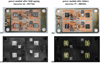 |
Fig. 1 Characterisation of failure mechanisms in inverter components, Top: (a & b): power modules without housing and encapsulation, bottom (c&d): non-destructive SAM analysis (wire bond plane) before removal of housing and encapsulation. |
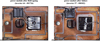 |
Fig. 2 Overview of the IGBTs shows the changes at emitter metallisation and wire bond connections after failure. |
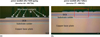 |
Fig. 3 Cross sectional view of the bonding wires and solder contact of DCB substrate (direct copper bonded) using light microscope imaging of the IGBTs. |
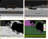 |
Fig. 4 Cross-sectional view of the melting area using SEM imaging (a) to (c) and EDX (d) for elemental analysis of the IGBTs from the power module after failure. |
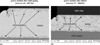 |
Fig. 5 Cross-sectional view of the solder contact using SEM imaging of the IGBTs. |
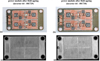 |
Fig. 6 Characterisation of failure mechanisms in inverter components, top (a&b): power modules without housing and encapsulation, bottom (c&d): non-destructive SAM analysis (overview module) before removal of housing and encapsulation. |
3.2 Impact analysis
3.2.1 Pattern of deviating inverter behaviour
Based on data pre-evaluation, an an unusual pattern indicating irregular inverter behaviour was identified, as displayed in Figure 7. The values shown are from two central inverters, are from PV Plant one and were installed in 2012. The characteristic of this pattern is that during a grid operator-induced curtailment to 0%, switches repeatedly between between different operating states, as seen in the parameter “PV state”. The inverter would normally switch to a specific “PV state” (derating (5)) and remain in this state until the curtailment is over (see inverter 8). Additionally, the AC currents of inverter 7 fluctuate between approximately 90 A and 0 A and the AC reactive power as well as small oscillations between 0 var and 10 var. After the curtailment ended, the inverter displayed an IGBT switching error message (see parameter “Inverter error”). The corresponding explanation of the inverter's status information is included in Table 3. For the present inverter type, different status information is distinguished for the control of the inverter, which is assigned to different functional groups.
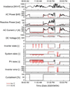 |
Fig. 7 Comparison of individual electrical measured variables and status information of inverter 7 (Inv 7) and a comparable inverter 8 (Inv 8) in the same PV plant 1, on 04.04.2020. |
Description of state parameters of the investigated inverter type.
3.2.2 Impact on system portfolio
The faulty inverter behaviour during curtailment, as described in the previous chapter was further investigated for the entire system portfolio.
The following questions were addressed.
How often does curtailment take place?
How many inverters show the observed pattern?
Do faults which point to the IGBT module occur in a temporal relationship to the curtailment?
To answer the first question, the states of the curtailment were summed up for each PV plant with a time resolution of one minute. Figure 8 (left) shows the number of curtailments determined for PV plant 2, subdivided by month and year. In addition, a further distinction was made here between curtailment due to the grid operator and an economically motivated direct marketing. As can be seen in the diagram, curtailment were relatively rare prior to until the beginning of 2021 but occurs very frequently from this point onwards. Furthermore, the system operator records the causes of system derating in different categories, it can be clearly seen that the PV plant was very rarely shut down for economic reasons, here i.e. direct marketing. The observations are also similar for PV plant one and PV plant three, which can be found in the appendix in Figures A1 and A2 of this article.
The second question, how many inverters show this irregular behaviour, can be answered by checking the “PV state”, which switches back and forth between different states during curtailment but should normally remain in one state (derating (5); see Tab. 3). A moving average with a window of two consecutive time steps was determined and used for this purpose. Whenever this number does not correspond to the desired status (derating (5), there is a deviating behaviour. If a deviating behaviour occurs, these time steps are summed up. The resulting number, aggregated per month and year, is demonstrated in Figure 8 (right) for every inverter in PV plant 2. Correlated to the occurrence of curtailment, this behaviour also appears very seldom until 2021 and only with a small number of inverters. From this point onwards, however, almost all systems follow this behaviour. The same observation also applies to the inverters in PV plant one and PV plant three, the diagrams of these are included in the appendix in Figures A1 and A2.
This leads to the third question: how frequently do error messages related to the IGBT module occur due to curtailment in this dataset. To check this, 7-days periods, starting in the same minute as curtailment starts and ending 7 days later, were separated from the entire dataset for all curtailment situations that occurred, and the error messages that appeared in these periods were summed up. The curtailment status itself is generally not a subject of the error categories. The period of 7 days was chosen to capture as many different weather situations as possible, in which the systems would perform differently.
All error messages occurring in these periods are shown in Figure 9, with the corresponding short description. Firstly, to provide a general overview of the error messages received: The error messages that appear in the list “no assignment possible” cannot be mapped to a description in the manufacturer's documentation, which makes it impossible to determine the cause. The number of error messages relating to grid quality or grid faults is remarkable and can be seen across all inverters, but these are not associated to the curtailment or IGBT failures. These error messages are self-clearing as soon as the grid quality is restored, but they prevent the inverters from feeding into the grid. Other messages are, for example, notifications when shutdowns have occurred due to maintenance work or faults in data transmission and software.
Secondly, more directly relevant the error messages that are relevant for the IGBT component to answer finally the third question: “IGBT overcurrent”, “IGBT switch-on error”, “Overtemperature error”. As can be seen in the diagram, these errors occur in some inverters, whereby even small numbers of occurrences can mean critical states. The same overview has also been created for the inverters in PV plant one and PV plant three and is documented again in the appendix in Figures A3 and A4. The answers to these three questions, based on the presented and explained diagrams and their correlations, show a clear relevance for the entire system portfolio.
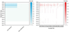 |
Fig. 8 Correlation of curtailments-related influences on inverters in PV plant 2. Counts are determined based on dataset with resolution of 1 min. Left: differentiation between the causes of curtailment and their monthly counts. Right: detected frequent status changes based on “PV state”. |
 |
Fig. 9 Number of error messages occurring in a seven-day period starting from the exact minute of each curtailment event and ending 7 days later for all curtailment situations in PV plant 2. |
3.2.3 Detection of pattern in monitoring data
This part of the study investigates whether it would have been possible to detect the described error pattern using machine learning methods without knowing them in advance.
The results of the different applied machine learning methods, described in the chapter “Material and Methods”, are shown below using data from an exemplary inverter from PV plant 2 for two consecutive years. The year 2021 was used to train the ANN. The trained model was then used to predict the DC and AC power for the year 2022. The clustering steps are solely related to the period of 2022. The year 2022 is of interest here because the faulty behaviour of the selected inverter occurred multiple times during this period.
The dataset and the associated parameter settings for the ANN modelling are shown in Table 2. Figure 10 is a scatter plot and shows the measured and predicted power for DC and AC for the period used for modelling. The certainty in terms of RMSE is for the modelling year 15.6 kW for DC power and 15.4 kW for AC power. While the model performs well across most of the power range, a noticeable bias is present in the lower range (up to approximately 25–50 kW, observed power). In this range, the ANN systematically overestimates power by an average of 25–50 kW. This discrepancy likely arises from the nature of data at low irradiance or low power levels, where nonlinearities and irregularities due to higher measurement uncertainties may lead to incorrect behaviour being learned by the model. Additionally, effects can be attributed to the inverter's own consumption, AC-DC imbalances and starting conditions of the inverter, which cannot be completely excluded in the training process. This ANN model can now be used to predict the expected output for the following year, using the ambient conditions as input.
This trained model performance can now be included as a reference in the cluster dataset to influence the formation of the clusters. This leads to the results of the first clustering, based on the dataset of 2022. The parameters and settings used are listed in Table 2. The results of the first cluster step are illustrated in Figure 11. The corresponding clusters for the ratio of the measured to the predicted power visualised in two colours: blue. The blue cluster represents the normal operating behaviour, and the points marked in gray represent deviating behaviour (outlier). Among other things, the two boundary areas are outliers appear concentrated in, for measured power levels around zero and for power levels above 500 kW. The deviations of the predicted outputs in the power range above 500 kW are because these high outputs were not present in the 2021 training data and an extrapolation for the model is not possible. This shows the limits of the ANN quite clearly.
To further differentiate the deviating behaviour, only the outliers are now included as a dataset in the second cluster step, still based on 2022. In addition, the clustering parameters are further reduced. An overview of the parameters and settings is provided in Table 2. The results of the second clustering are shown in Figure 12. Since only DC parameters are used for the second clustering step (as shown in Tab. 2), the analysis shifts from AC power in Figure 11 to DC current in Figure 12. The choice of AC or DC parameters is based on the need to best visualise the clustering results and dependencies, ensuring a clearer differentiation of operational states. The clustering resulted in 20 finer clusters (0 to 19), which make up 35% of this specific dataset, the rest is noise. Due to the clearly visible structure and separability, clusters can be grouped into areas. For the sake of simplicity, we have used in this plot (Right) the same colors for clusters that belong to the same area.
The clusters form different separated areas: 1, 2, 3, 4, 5, and 6. The formation of the cluster in area 2 is particularly important here, as it is related to the error pattern as observed and described in chapter 0. These individual cluster areas can be explained using specific visualisations, ideally in 2 or 3 dimensions. Such helpful diagrams are collected in Figure A.5, in Appendix A. It is important to note that there were no error messages from the inverter in this dataset. The results from the second clustering obtained in this study, based on the systems evaluated, can be described as follows:
Area 1 (consists of cluster 0, 1, 2, 3, and 4): The clusters occur primarily in winter or spring, accompanied by low irradiance values. The data occurs more frequently towards midday, which means that this could be due to a possible performance reduction caused by partial shading or snow. The ambient temperatures are below 5 °C (except cluster 0). TMatrix is different for each cluster: 15–35 °C (clusters 0 and 2), 37–47 °C (3), and 50–57 °C (4). Cluster 4 is in the normal TMatrix operating range. All clusters of this area only occur when the inverter is in normal operating mode and there are no curtailments as indicated by the system status.
Area 2 (Cluster 7, 14, 16, 17, 18, and 19): This area is generally characterised by low DC current and low DC power even though sufficient irradiance would be available. The observed error pattern belongs to 16, 17, 18 and 19: different “PV states” appear in these clusters during curtailment, as observed in the error pattern. The high number of clusters is due to different voltage levels that lie in the open-circuit voltage range (>650 V). Cluster 19 is also separated due to high ambient temperature of more than 35 °C. Even though the values of clusters 7 and 14 are very close to the previously mentioned clusters, correspond to standby or normal operation standby and normal operating mode, in which there is no curtailment.
Area 3 (Cluster 5, 6, and 10): The clusters occur on a few days, more often in the morning and midday hours. The ambient temperature is below 5 °C, but the TMatrix is normal 50–60 °C. Furthermore, these clusters show less scattering for example compared to area 1. A separated voltage range is appearing: 610–640 V. To summarise, these clusters can be classified as normal operation at cold temperatures and low irradiances. Concerning the system status, these clusters appear solely when the inverter is operating in normal mode and no curtailments are present.
Area 4 (Cluster 15): This cluster occurs mainly in the summer mornings, at ambient temperatures between (15–30 °C) and normal matrix temperature (45–60 °C). The voltage range is 525–580 V and the power is high, despite moderate irradiance values. There could be higher weather dynamics here, e.g. passing clouds. The system status corresponds to normal operating mode, and curtailments do not occur.
Area 5 (Cluster 11, 12, and 13): These clusters are similar to area 4, the ambient temperature is in the range of (10–30 °C), with a normal temperature-voltage behaviour (the values are on the voltage-temperature regression line). The matrix temperature is in the normal range of (50–60 °C), with a lower voltage range of (480–580 V). The main cluster assessment would be: weather-related deviations under normal behaviour. The system status reflects normal operating mode, with no curtailments taking place.
Area 6 (Cluster 8 and 9): These clusters occur at high irradiance levels at midday, with warm ambient temperatures 25–35 °C (difference: cluster 9 > 30 °C, cluster 8 < 30 °C). The voltage values are lower, whereas the matrix temperature is in a normal range (52–58 °C). These are special cases that occur during normal operating behaviour at high ambient temperatures and low operating voltages. These two clusters also occur in normal operating mode without curtailments.
As illustrated by the detailed assessments of the clusters, clustering is not a self-sustaining process; rather, the subsequent interpretation is crucial, particularly during method development. This evaluation aids in distinguishing between critical and non-critical states. The observed error pattern could clearly be categorised into four clusters (cluster 16, 17, 18, 19), which differ solely based on varying voltage levels and ambient temperatures. Although the status information and curtailment data were not included as parameters during clustering, the process was still able to distinguish between them due to subtle nuances among the multidimensional parameters, considering ANN prediction as references in the first clustering step.
The presence of these clearly identified areas in the dataset can be automatically validated in newly clustered time periods (comparable inverter devices or years, with same available parameters) through the use of classification algorithms. This enables a targeted search for problematic performance behaviour of interest in monitoring data and furthermore the determination of statistical frequencies of such events. This helps operators to compare the operating behaviour of devices and to evaluate action measures for failures more quickly.
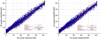 |
Fig. 10 Training of ANN. Comparison between measured (observed) and predicted power of year 2021, including a linear regression with intercept set to zero. Left: DC power training accuracy. Right: AC power of training accuracy. |
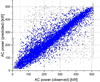 |
Fig. 11 Result of 1st clustering, applied to the dataset of 2022. Blue: Main cluster representing normal inverter behaviour (89% of total dataset). Gray: Irregular behaviour or outliers (11% of total dataset). |
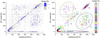 |
Fig. 12 Result of second clustering, applied to the data marked as outlier from first clustering of year 2022. The scale indicates the number of the cluster. Left: Entire dataset including outliers (gray). Right: As left, but excluding outliers and with defined cluster areas (1 to 6). |
4 Discussion
The results of the interdisciplinary investigation, utilising methodologies from materials science, data analysis, statistics, and machine learning, fit together and complete each other. The assumed mechanism, based on materials science, is that a prolonged temperature impact during the application led to the degradation of the semiconductors and thus to an increasing overload. This overload, which the components are exposed to over a longer period, corresponds to the detected error pattern of the inverter to enter in undefined states during the curtailment. This usually occurs in the late morning and midday and persists for several hours or even longer if grid maintenance is taking place. Due to the overall increase in curtailment times, the power components are increasingly exposed to the conditions leading to failure. Furthermore, indications in the form of error messages pointing to the IGBT components were found in varying numbers in the system portfolio in temporal correlation to the curtailments. And concerning the question of being able to recognise such deviations in automated form, even without prior knowledge, an innovative concept was presented that was able to differentiate the error pattern in the dataset in several steps using different machine learning methods.
The clustering methodology plays a significant role in this context, enabling the identification of recurring inverter behaviour patterns beyond traditional threshold-based filtering. It takes into account multi-parametric correlations of electrical and environmental data in high resolution in order to break them down into times with similar characteristics. This approach goes beyond conventional filtering methods as non-linear correlations and frequencies in multi-dimensional data are taken into account in the search for inverter malfunctions. In addition, precise filter criteria do not have to be known from the outset, which may vary depending on the technical specifications, location and seasons of the year. Clustering also makes it possible to find unknown phenomena that might otherwise not have been recognised by targeted filtering.
In the first step presented, clustering successfully differentiated between “normal” and “deviating” behaviour. Within the latter, additional substructures of repeating patterns were identified, providing deeper insights into operational inconsistencies. While the current clustering approach primarily distinguishes operational states based on environmental parameters such as irradiance, ambient and matrix temperature, as well as DC parameters, its value lies in detecting underlying behavioural anomalies that might otherwise go unnoticed. A detailed analysis of these clusters (as shown in Fig. 12) reveals deviating behaviour under various environmental and operational conditions.
For example, area 2 is particularly significant as it is directly related to the error pattern shown in Figure 7 and described in Chapter 3.2.1. This area is characterised by low DC current and low DC power levels, even when sufficient irradiance is available. Within this category, clusters 16, 17, 18, and 19 exhibit different “PV states” during curtailment, aligning closely with the observed failure pattern. Additionally, different voltage levels within the open-circuit voltage range (>650 V) contribute to the distinct classification of these clusters. The presence of cluster 19 at ambient temperatures exceeding 35 °C further emphasises that temperature influences inverter behaviour during curtailment periods. Other areas provide important operational insights as well: clusters in area 1 mainly occur in winter and early spring, with low irradiance values and ambient temperatures below 5 °C. These could be linked to partial shading or snow accumulation, as they are observed more frequently around midday.
These findings illustrate that clustering is not just a data filtering tool but a powerful diagnostic approach for distinguishing between critical and non-critical inverter operation. By systematically defining parameters within suitable frameworks − especially in multidimensional data contexts − future clustering iterations can automate the search for these specific failure patterns across large datasets. Refining the clustering process to incorporate additional features, such as power ramp rates or curtailment duration, could enhance the detection of operational inconsistencies across multiple inverters. Expanding this approach to a broader system portfolio could provide valuable insights into the systemic impact of curtailment events on inverter reliability. Future work should therefore explore advanced clustering techniques to increase differentiation and improve predictive capabilities, enabling more targeted diagnostic and preventive strategies.
The crucial question now is how this behaviour of the inverter can be corrected. This deviation has an enormous impact on the entire system portfolio in the long or short term. It is also reasonable to assume that far more systems in which this type of inverter has been installed may be affected. The curtailment itself cannot be avoided. However, where should the error be found? Is it in the inverter software or in a faulty signal transmission? In terms of intervening in the inverter software, it is not possible because the product is no longer being developed. Regarding signal transmission, there are ten power modules mounted per phase, and the control signal is looped through all of them. The greatest deviations would be expected at the last segment in the chain. Unfortunately, there are limits to the data analysis here, as no high-resolution information is available on the functional groups involved. The available results only manage to narrow this problem but cannot solve it. Possible corrective measures must be evaluated and implemented in the PV plant itself.
5 Conclusion
The aspect of curtailment is important to consider from the authors' perspective, as it is expected to occur more frequently in the near future. It is necessary to assess the extent to which inverters can enter the intended state or whether regulation-related issues arise, which can be verified, for example, through inverter status information. Are the processes always the same, or do they change dynamically over time? Additionally, it is useful to check whether error messages occur more frequently in temporal correlation with curtailments, as such patterns may indicate underlying control or operational issues.
To effectively monitor larger system portfolios, it is important to define a target operational state for each system, as demonstrated through the ANN-based approach in this study. Comparing this expected behaviour with the currently measured values enables automated detection of deviations. To better differentiate deviations in the next step, the OPTICS clustering method has proven to be a valuable tool for systematically identifying distinct operational states and failure patterns.
From our authors' perspective, beyond operational monitoring, it is also important to strengthening research at the material level, in combination with real-world stress conditions in the field, through intensive data analysis. This interdisciplinary approach will allow for more precise statements regarding the ageing and potential failures of components and functional groups. For example, quantifying the percentage of efficiency loss in inverters due to specific stress factors would provide value in predicting ageing and degradation trends and optimising long-term system reliability.
The proposed approach provides a systematic concept for PV monitoring, enhancing predictive maintenance and reducing costly reactive O&M. These findings also offer valuable insights for inverter manufacturers, supporting firmware improvements against curtailment-related stress factors. While this study focused on a specific portfolio, the methodology is scalable to larger or more diverse PV fleets, adapting to different inverter models, climatic conditions, and system configurations. Future research should explore more advanced clustering techniques or hybrid models that integrate material and data-driven diagnostics with physical simulations. Additionally, expanding material-level research to long-term degradation modelling will further improve the predictive accuracy of inverter failure assessments, strengthening system reliability for the evolving renewable energy landscape.
Glossary
Term: Definition
ADAM: Adaptive moment estimation
Ag: Silver
ANN: Artificial neural network
Al: Aluminum
Cu: Copper
DBSCAN: Density-based spatial clustering of applications with noise
DCB: Direct copper bonded
EDX: Energy dispersive X-ray spectroscopy
IGBT: Insulated-gate bipolar transistor
OPTICS: Ordering points to identify the clustering structure
MTTD: Mean time to detect
MTTR: Mean time to repair
ReLU: Rectified linear unit
SAM: Scanning acoustic microscopy
SEM: Scanning electron microscopy
Si: Silicon
Sn: Tin
Funding
This research was funded in the “robStROM” project by the Federal Ministry for Economic Affairs and Climate Action in Germany as part of the 7th Energy Research Program (funding code: 03EE1163B). The institutions of Deutsche Solarservice GmbH, Fraunhofer Institute for Microstructure of Materials and Systems and DENKweit GmbH have received funding in the project “robStROM” from the Federal Ministry for Economic Affairs and Climate Action in Germany as part of the 7th Energy Research Program (funding code: 03EE1163B).
Conflicts of interest
All authors certify that they have no financial conflicts of interest (e.g., consultancies, stock ownership, equity interest, patent/licensing arrangements, etc.) in connection with this article.
Data availability statement
Data associated with this article cannot be disclosed due to legal reason. All monitoring data from the photovoltaic systems used in this project are anonymised in the sense of location, owner, etc. The typus of the inverter for the root cause analysis is also anonymised in this paper.
Author contribution statement
Conceptualisation: Andreas Dietrich, Carsten Hennig, Danny Wehnert. Methodology: David Daßler, Stephanie Malik, Carola Klute, Robert Klengel. Software: Kai Kaufmann, David Daßler, Stephanie Malik, Dharm Patel. Validation: David Daßler, Stephanie Malik. Data curation: Kai Kaufmann, Dharm Patel. Writing − review and editing: Stephanie Malik, David Daßler, Carola Klute, Robert Klengel. Writing − Review & Editing: Dharm Patel, Matthias Ebert. Visualisation: Carola Klute, Robert Klengel, David Daßler. Supervision: Andreas Dietrich, Kai Kaufmann, Carsten Hennig, Danny Wehnert, Matthias Ebert. Project Administration: Andreas Dietrich.
References
- P. Hacke, S. Lokanath, P. Williams, A. Vasan, P. Sochor, G. TamizhMani, H. Shinohara, S. Kurtz, A status review of photovoltaic power conversion equipment reliability, safety, and quality assurance protocols, Renew. Sustain. Energy Rev. 82 1097 (2018). https://doi.org/10.1016/j.rser.2017.07.043 [CrossRef] [Google Scholar]
- A. Golnas, PV system reliability: An operator's perspective, IEEE J. Photovolt. 3, 1 (2013). https://doi.org/10.1109/JPHOTOV.2012.2215015 [Google Scholar]
- J.M. Freeman, G.T. Klise, A. Walker, O. Lavrova, Evaluating energy impacts and costs from PV component failures, in 2018 IEEE 7th World Conference on Photovoltaic Energy Conversion (WCPEC) (A Joint Conference of 45th IEEE PVSC, 28th PVSEC & 34th EU PVSEC) (2018). https://doi.org/10.1109/PVSC.2018. 8547454 [Google Scholar]
- VDMA, International Technology Roadmap for Photovoltaic (ITRPV) − 2022 Results, 14th edn. (2023) [Google Scholar]
- J. Falck, C. Felgemacher, A. Rojko, M. Liserre, P. Zacharias, Reliability of power electronics systems: An industry perspective, IEEE Ind. Electron. Mag. 12, 24 (2018). https://doi.org/10.1109/MIE.2018.2825481. [Google Scholar]
- M. Shahzad, K.V.S. Bharath, M.A. Khan, A. Haque, Review on reliability of power electronic components in photovoltaic inverters, in 2019 International Conference on Power Electronics, Control and Automation (ICPECA) (2020). https://doi.org/10.1109/ICPECA47973.2019.8975585 [Google Scholar]
- A. Sangwongwanich, Y. Yang, D. Sera, F. Blaabjerg, Mission profile-oriented control for reliability and lifetime of photovoltaic inverters, IEEE Trans. Ind. Appl. 56, 1 (2020). https://doi.org/10.1109/TIA.2019.2947227 [Google Scholar]
- SolarPower Europe, Global Market Outlook for Solar Power 2024–2028 (SolarPower Europe, 2024) [Google Scholar]
- J. Leloux, Mapping the Relevance of Digitalisation for Photovoltaics, in Intersolar Conference (2024) [Google Scholar]
- SolarPower Europe, Operation & Maintenance: Best Practice Guidelines, Version 5.0 (2021) [Google Scholar]
- IEA-PVPS, Guidelines for Operation and Maintenance of Photovoltaic Power Plants in Different Climate Zones, Report IEA-PVPS T13-25:2022 (2022) [Google Scholar]
- A. Livera, M. Theristis, L. Micheli, E.F. Fernández, J.S. Stein, G.E. Georghiou, Operation and maintenance decision support system for photovoltaic systems, IEEE Access 10, 42481 (2022). https://doi.org/10.1109/ACCESS.2022.3168140 [CrossRef] [Google Scholar]
- D. Daßler, S. Malik, S.B. Kuppanna, B. Jäckel, M. Ebert, Innovative approach for yield evaluation of PV systems utilising machine learning methods, in 46th IEEE PVSC (Chicago, 2019). https://doi.org/10.1109/PVSC40753.2019.8981367 [Google Scholar]
- D. Daßler, S.B. Kuppanna, S. Malik, R. Schmidt, M. Ebert, Training and evaluation for yield-driven detection of losses in PV systems utilising artificial neural networks, in IEEE 47th Photovoltaic Specialists Conf. (PVSC) (Virtual, 2020) https://doi.org/10.1109/PVSC45281.2020.9300490 [Google Scholar]
- G.D. Rupakula, D. Daßler, S. Malik, M. Ebert, R. Schmidt, Automatic fault detection and classification in PV systems by the application of machine learning algorithms, in 38th Eur. Photovolt. Sol. Energy Conf. and Exhibition (2021). https://doi.org/10.4229/EUPVSEC20212021-5DO.1.2 [Google Scholar]
- D. Daßler, S. Malik, R. Gottschalg, M. Ebert, Effect of availability and quality of data on the detection of defects utilising artificial neural networks in PV system monitoring data, in 8th World Conf. on Photovolt. Energy Conv. (Milan, 2022). https://doi.org/10.4229/WCPEC-82022-4DO.1.5 [Google Scholar]
- Deutscher Wetterdienst, CDC (Climate Data Center), accessed 17 May 2024. https://www.dwd.de/DE/klimaumwelt/cdc/cdc_node.html [Google Scholar]
- S. Malik, D. Daßler, J. Fröbel, J. Schneider, M. Ebert, Outdoor data evaluation of half-/full-cell modules with regard to measurement uncertainties and the application of statistical methods, in 29th Eur. Photovolt. Sol. Energy Conf. and Exhibition (Amsterdam, 2014) [Google Scholar]
- M. Ankerst, M.M. Breunig, H.-P. Kriegel, J. Sander, OPTICS: ordering points to identify the clustering structure, ACM SIGMOD Rec. 28, 49 (1999) [CrossRef] [Google Scholar]
- E. Schubert, M. Gertz, Improving the cluster structure extracted from OPTICS plots, in Proc. Conf. “Lernen, Wissen, Daten, Analysen” (LWDA, 2018) pp. 318–329 [Google Scholar]
- F. Pedregosa et al., Scikit-learn: Machine learning in Python, J. Mach. Learn Res. 12, 2825 (2011) [Google Scholar]
- Reprint of: P.C. Mahalanobis, On the generalised distance in statistics (Sankhya A 80, Suppl. 1, 2018) pp. 1–7. https://doi.org/10.1007/s13171-019-00164-5 [Google Scholar]
Cite this article as: Stephanie Malik, David Daßler, Dharm Patel, Carola Klute, Robert Klengel, Andreas Dietrich, Kai Kaufmann, Carsten Hennig, Danny Wehnert, Matthias Ebert, Analysis of fault detection and defect categorisation in photovoltaic inverters for enhanced reliability and efficiency in large-scale solar energy systems, EPJ Photovoltaics. 16, 25 (2025), https://doi.org/10.1051/epjpv/2025011
Appendix A
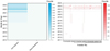 |
Fig. A1 Comparison for 2nd set of inverters (PV plant 1): correlation of curtailments-related influences on inverters. Left: differentiation between the causes of curtailment and their monthly counts. Right: detected frequent status changes based on “PV state”. |
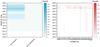 |
Fig. A2 Comparison for 3rd set of inverters (PV plant 3): correlation of curtailments-related influences on inverters. Left: differentiation between the causes of curtailment and their monthly counts. Right: detected frequent status changes based on “PV state”. |
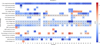 |
Fig. A3 Number of error messages occurring in a 7-days period starting in the same minute as curtailment starts and ending 7 days later for all curtailment situations in PV plant 1. |
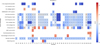 |
Fig. A4 Number of error messages occurring in a 7-days period starting in the same minute as curtailment starts and ending 7 days later for all curtailment situations in PV plant 3. |
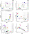 |
Fig. A5 Supplementary types of representation of the results from 2nd Clustering. |
All Tables
Overview of the available parameters per inverter (area: inverter) and per system (system status and environment). The values are available at a 1-minute time resolution.
All Figures
|
Fig. 1 Characterisation of failure mechanisms in inverter components, Top: (a & b): power modules without housing and encapsulation, bottom (c&d): non-destructive SAM analysis (wire bond plane) before removal of housing and encapsulation. |
| In the text | |
|
Fig. 2 Overview of the IGBTs shows the changes at emitter metallisation and wire bond connections after failure. |
| In the text | |
|
Fig. 3 Cross sectional view of the bonding wires and solder contact of DCB substrate (direct copper bonded) using light microscope imaging of the IGBTs. |
| In the text | |
|
Fig. 4 Cross-sectional view of the melting area using SEM imaging (a) to (c) and EDX (d) for elemental analysis of the IGBTs from the power module after failure. |
| In the text | |
|
Fig. 5 Cross-sectional view of the solder contact using SEM imaging of the IGBTs. |
| In the text | |
|
Fig. 6 Characterisation of failure mechanisms in inverter components, top (a&b): power modules without housing and encapsulation, bottom (c&d): non-destructive SAM analysis (overview module) before removal of housing and encapsulation. |
| In the text | |
|
Fig. 7 Comparison of individual electrical measured variables and status information of inverter 7 (Inv 7) and a comparable inverter 8 (Inv 8) in the same PV plant 1, on 04.04.2020. |
| In the text | |
|
Fig. 8 Correlation of curtailments-related influences on inverters in PV plant 2. Counts are determined based on dataset with resolution of 1 min. Left: differentiation between the causes of curtailment and their monthly counts. Right: detected frequent status changes based on “PV state”. |
| In the text | |
|
Fig. 9 Number of error messages occurring in a seven-day period starting from the exact minute of each curtailment event and ending 7 days later for all curtailment situations in PV plant 2. |
| In the text | |
|
Fig. 10 Training of ANN. Comparison between measured (observed) and predicted power of year 2021, including a linear regression with intercept set to zero. Left: DC power training accuracy. Right: AC power of training accuracy. |
| In the text | |
|
Fig. 11 Result of 1st clustering, applied to the dataset of 2022. Blue: Main cluster representing normal inverter behaviour (89% of total dataset). Gray: Irregular behaviour or outliers (11% of total dataset). |
| In the text | |
|
Fig. 12 Result of second clustering, applied to the data marked as outlier from first clustering of year 2022. The scale indicates the number of the cluster. Left: Entire dataset including outliers (gray). Right: As left, but excluding outliers and with defined cluster areas (1 to 6). |
| In the text | |
|
Fig. A1 Comparison for 2nd set of inverters (PV plant 1): correlation of curtailments-related influences on inverters. Left: differentiation between the causes of curtailment and their monthly counts. Right: detected frequent status changes based on “PV state”. |
| In the text | |
|
Fig. A2 Comparison for 3rd set of inverters (PV plant 3): correlation of curtailments-related influences on inverters. Left: differentiation between the causes of curtailment and their monthly counts. Right: detected frequent status changes based on “PV state”. |
| In the text | |
|
Fig. A3 Number of error messages occurring in a 7-days period starting in the same minute as curtailment starts and ending 7 days later for all curtailment situations in PV plant 1. |
| In the text | |
|
Fig. A4 Number of error messages occurring in a 7-days period starting in the same minute as curtailment starts and ending 7 days later for all curtailment situations in PV plant 3. |
| In the text | |
|
Fig. A5 Supplementary types of representation of the results from 2nd Clustering. |
| In the text | |
Current usage metrics show cumulative count of Article Views (full-text article views including HTML views, PDF and ePub downloads, according to the available data) and Abstracts Views on Vision4Press platform.
Data correspond to usage on the plateform after 2015. The current usage metrics is available 48-96 hours after online publication and is updated daily on week days.
Initial download of the metrics may take a while.