| Issue |
EPJ Photovolt.
Volume 17, 2026
Special Issue on ‘EU PVSEC 2025: State of the Art and Developments in Photovoltaics', edited by Robert Kenny and Carlos del Cañizo
|
|
|---|---|---|
| Article Number | 17 | |
| Number of page(s) | 16 | |
| DOI | https://doi.org/10.1051/epjpv/2026010 | |
| Published online | 24 April 2026 | |
https://doi.org/10.1051/epjpv/2026010
Original Article
Maps of long-term soiling losses in Europe considering a partial cleaning effect by rain
1
German Aerospace Center (DLR), Institute of Solar Research, Calle Doctor Carracido, 44, 04005 Almería, Spain
2
Sapienza University of Rome, Department of Astronautical, Electrical and Energy Engineering (DIAEE), 00184 Rome, Italy
3
University of Almería, Department of Chemistry and Physics, Carretera Sacramento s/n, 04120 La Cañada de San Urbano, Almería, Spain
4
Centro de Investigaciones Energéticas, Medioambientales y Tecnológicas (CIEMAT), Photovoltaic Solar Energy Unit, Avda. Complutense 40, 28040 Madrid, Spain
5
Centro de Investigaciones Energéticas, Medioambientales y Tecnológicas (CIEMAT), Energy Department – Renewable Energy Division, Avda. Complutense 40, 28040 Madrid, Spain
* e-mail: This email address is being protected from spambots. You need JavaScript enabled to view it.
Received:
30
September
2025
Accepted:
18
March
2026
Published online: 24 April 2026
Abstract
The soiling of PV modules has been estimated to yield global losses in the solar energy production by 4 to 7%, even considering the cleaning efforts in many solar energy systems. Despite this, soiling measurements are not always available, making models particularly valuable for estimating these losses. However, soiling models currently present two limitations: most of them assume that daily rain accumulations higher than a threshold value can totally clean PV modules and, additionally, that rain will have the same washing effect on all types of soiling, independently of their higher or lower adherent properties. In this work, the HSU model (Coello and Boyle, 2019) is modified to include the two aforementioned effects. The original and modified HSU models are then calibrated for two locations in Africa where observations of long-term soiling losses were available. At the first considered location, the predominant soiling type was mainly washable by rain but showed the partial cleaning effects, while at the second location, despite the frequent and abundant rainfall, the build-up of persistent soiling was observed. The calibrated parameters for the original and modified HSU models were then applied to reanalysis meteorological 2-dimensional input data to estimate the associated soiling losses in Europe for a 20-yr operation without any artificial cleaning. The application of model parameters derived for the African sites for Europe is considered to be valid for the demonstration of the method and delivers exemplary results that might also occur for soiling types found at some European sites. The derived different soiling maps should, however, not be understood as the most likely possible values for European soiling. When considering the exemplary removable soiling type, the original HSU model underestimates on average the European soiling losses by a factor of 4 compared to the estimations of the modified HSU model. When considering the exemplary persistent soiling type, the European soiling losses estimated with the modified HSU model are on average 5.5 times larger than those estimated with the original HSU model. Additionally, the European soiling losses estimated with the modified HSU model considering a persistent soiling type are 2.4 times larger than those considering a removable soiling type, which highlights not only the importance of properly modeling the soiling losses but also of choosing the correct soiling type. The results show that, at least for some soiling types, mechanical cleaning of the PV modules is necessary to avoid high soiling losses even in rainy regions such as Central Europe.
Key words: Soiling modelling / model optimization / soiling maps / cleaning by rain
These authors contributed equally to this work.
© E. Ruiz-Donoso et al., published by EDP Sciences, 2026
 This is an Open Access article distributed under the terms of the Creative Commons Attribution License (https://creativecommons.org/licenses/by/4.0), which permits unrestricted use, distribution, and reproduction in any medium, provided the original work is properly cited.
1 Introduction
Soiling is defined as the accumulation of pollutants on top of photovoltaic (PV) panels. Global losses in energy production have been reported to reach 4 to 7%, even with regular cleaning efforts at many solar energy systems [1]. The losses of individual PV installations can deviate from the stated interval, depending, among other influences, on the specific location, local soiling sources, the PV technology, and the cleaning schedule. At locations with high levels of precipitation, the natural cleaning effect by rain might keep the PV modules sufficiently clean [2], and the frequency of manual or automated cleaning might be reduced. Correctly identifying the correct schedule for the manual or automated cleaning can result in a significant economic saving [3–6]. In order to correctly characterize the degree of cleaning achieved by the rain at one specific location and hence identify the most appropriate manual cleaning frequency, the analysis of long-term trends of soiling losses is necessary [7].
Observations of long-term trends of soiling losses are scarce, and only a comparably small fraction of soiling studies investigates soiling data sets longer than a year without frequent cleaning [8,9]. Hence, soiling models play an important role in this regard. However, previous works have already highlighted several limitations in the state-of-the-art soiling models. Physical models estimate the soiling loss corresponding to the mass deposited on a PV panel under certain meteorological conditions taking into consideration the PV modules' tilt angle. They assume a total cleaning of the PV panels by rain (i.e., a soiling loss of 0% after the rain) after a day with a rain sum higher than a given threshold [10,11]. Based on experimental data, Hanrieder et al. [12] pointed out the inaccuracy of this assumption: partial cleaning by rain occurs often, and low daily rain sums can also clean the PV modules up to a certain degree. Valerino et al. [13] used the hourly rainsum and reported that rainfall <5 mm/h does not fully clean modules. Norde Santos et al. [14] suggested a natural cleaning model, in which the effectiveness of natural partial cleaning of PV modules depends on the parameters related to soiling and the rain episode itself. The simple threshold-based approach was also enhanced in [15] by assuming that 80% of the soiling particles are washed away for rain events with >10 mm rain sum and 30% for <5 mm. Li et al. [16] assumed that for <1 mm/h rain does not clean, but >5 mm/h reaches full cleaning, and introduced thresholds for which specific soiling particles are fully or partly removed (1 to 3 mm/h: sulfate fully cleaned, half of the organic carbon removed; 3 to 5 mm/h: sulfate fully cleaned, half of all other particles are removed).
Even after these model enhancements, nearly all currently available soiling models do not consider soiling species that firmly adhere to the PV module and cannot be removed by rain. This is an important shortcoming, as all of the above models predict close to zero soiling after several strong rain events. Hence, they cannot describe the long-term build-up of soiling layers. This kind of soiling appears at locations close to railroads, roads, or specific factories or affected by high concentrations of pollen and produces soiling losses of significant value even when frequent and abundant precipitation occurs. This type of soiling was reported in [9,17,18] and supports the inclusion of persistent soiling in model approaches. Assuming a continuous source of this kind of soiling, the associated PV soiling loss found after strong rain events is expected to steadily increase over time, unless the PV modules are manually cleaned. An important step forward in this regard was presented in [19], where PM2.5 (particulate matter with a diameter <2.5 µm) was assumed to contribute to non-removable soiling while the PM2.5–10 particles, with diameters between 2.5 and 10 µm, were assumed to be removable by rain. However, using only the diameter of the particles to describe if rain is able to remove them from the PV panel is still a rough assumption. Another model that used a fixed remaining soiling level that cannot be removed by rain was presented in [20]. There, improved versions of the HSU and Kimber models were introduced, including partial and incomplete rainfall cleaning that significantly improved model accuracy. However, their model with non-removable soiling used one fixed value of the soiling loss after strong rain cleaning for the whole time series, which cannot describe a continuous build-up of a soiling layer during several years of PV operation without cleaning.
Models also have the capabilities of estimating soiling losses at remote locations where no observations are available. This capability can be used to estimate the 2-dimensional (2D) distribution of soiling losses, thus generating soiling maps. This provides a valuable resource to stakeholders during the decision-making processes related to yield assessment, maintenance planning, resource optimization, and environmental impact assessment. For example, Fernández Solas et al. [17] presented a first estimation of the soiling losses at the European level, considering yearly cleaning in a state-of-the-art soiling model and a model describing partial cleaning by rain, which was described by a constant degree of partial cleaning, and did not consider the presence of persistent soiling highly adhered to the PV modules. Soiling maps for other regions such as the US have also been published, and uncertainties related to the input data and the modeling approach have been discussed [21].
In this work, a state-of-the-art soiling model is modified to incorporate the most recent findings: The widely used HSU soiling model [22] is enhanced to incorporate a partial cleaning effect by rain dependent on the rainsum and the possible presence of persistent soiling accumulating on the PV module. The modified and original model versions are calibrated with a novel set of soiling data in order to then produce maps of long-term trends of soiling losses in Europe. Each map represents the soiling losses for a specific exemplary soiling type with a given rain cleaning effect. The derived different soiling maps are examples of soiling types that might be found at some European sites. The maps hence demonstrate the method and illustrate the range of soiling losses that have to be expected for different soiling types. The maps should, however, not be understood as the most likely possible values for European soiling. The results produced by both models are compared to each other and to results from the literature, and their uncertainty is discussed.
The paper is organized as follows: Section 2 introduces the observations used in this study and presents the original and modified versions of the soiling model. In Section 3, the model is calibrated to the soiling type observed at two specific locations. Thereafter, average maps of 20-yr trends of soiling losses in Europe are presented, estimated with both model versions for the two considered soiling types. Section 4 elaborates on the main findings and conclusions.
2 Data and methods
This section describes the data used in this study and the methodology applied to it. Section 2.1 describes the ground-based observations collected at the East African Power Pool (EAPP) stations and the procedure to obtain daily soiling losses. Section 2.2 describes the two soiling models employed in this analysis: the original HSU model presented by [22] and a novel approach hereon referred to as HSU modified.
2.1 Observations from EAPP Stations
The World Bank launched a multi-location renewable-energy measurement project with financial support in the Energy Sector Management Assistance Program (ESMAP) to assist the East African Power Pool (EAPP) in conducting detailed renewable-energy resource assessments. The project concentrated on sites considered for large-scale solar power plant development in the near future and conducted a field campaign, implemented by GeoSUN Africa, where nine measurement stations were distributed across Kenya, Tanzania, and Uganda (Fig. 1). The campaign reports for each station are available at [23].
Each station was equipped with instrumentation to record several meteorological variables. In addition, each station consisted of three reference cells with a tilt angle of 10°, facing north at stations located in the southern hemisphere and facing south otherwise. They recorded the short-circuit current with a minute resolution between 15 December 2019 and 31 December 2021. One of the reference cells was cleaned daily, and its observations are considered the “clean reference”; the second one was cleaned with a monthly frequency, and the third one was left uncleaned during the complete campaign period. In this study, the measurements from both the pluviometer, for daily rain sums, and the PV reference cells, for soiling losses, are also considered.
The observations of the daily-cleaned reference cell and the uncleaned one were considered to evaluate the natural variability of the soiling losses (i.e., no manual cleaning is applied, and the only considered cleanings are those due to the rain effect) over the course of the campaign (2020–2021). Soiling ratios (SR) with 1 min resolution were calculated as:
 (1)
(1)
with Isoiled and Iclean being the short-circuit currents of the clean and soiled reference cell, respectively. The currents were calibrated relative to each other to yield a soiling ratio equal to 1 if both cells are clean. A temperature correction was also applied. The minutely resolved soiling ratios were transformed to daily soiling ratios following the methodology described by [24]. In a first step, the one-minute soiling ratios were filtered to eliminate outliers, and datapoints outside a reasonable range of 0.7 to 1.1 were discarded [24]. Values outside this range probably indicate sensor malfunction or the presence of strong localized soiling, such as bird droppings or tree leaves. Once the outliers are discarded, the daily data spread is assessed, and only measurements comprised between the daily 5th and 95th percentage are considered acceptable. Finally, a flattening adjustment compensates for systematic errors associated to the different orientation of the two sensors:
 (2)
(2)
where  corresponds to the flattened SR;
  corresponds to the observed SR; f(AZM) is a linear fit of
 with respect to solar azimuth angle over the course of the considered day; and f(180°) is the function's value at solar noon. To calculate the daily SR, only data within a time interval of 2 h around the solar noon is considered. The daily soiling loss in percent is given by
 (3)
(3)
For a given day, the accumulated rain sum is calculated as the cumulative rainfall occurring between 2 h after the solar noon of the previous day and 2 h after the solar noon of the current day. This corresponds to the time period affecting the observed soiling losses and ensures that the cleaning effect of the rain is accurately reflected in the SL measurements.
For this study, the soiling losses observed at the stations of Shinyanga (Tanzania) and Homa Bay (Kenya) are considered. The location of both stations is highlighted in green in Figure 1a. The measured soiling losses of the reference cell that was never cleaned are shown, along with the observed daily rain sums in Figure 2a for Shinyanga and in Figure 2b for Homa Bay. The climate at both stations is clearly different. Homa Bay is a tropical wet hot summer Köppen–Geiger climate [25], and Shinyanga is a tropical wet and hot semi-arid [26]. While both stations present large daily rain sums, in Shinyanga, they are distributed among the rainy season between mid-October and mid-April and the dry season during the rest of the year. Daily rain sums during the rainy season often surpass 20 mm day‒1 and can reach up to 80 mm day−1. In contrast, Homa Bay is affected by precipitation evenly distributed throughout the year and does not show different rainy and dry seasons. The daily rain sums are typically above 10 mm day−1 and can reach up to 50 mm day−1. This situation impacts the pattern of soiling losses observed at each station: during the dry season, Shinyanga's soiling losses steadily increase over time until the beginning of the rainy season, where the soiling losses decrease due to the cleaning effect of the rain. However, despite the large daily rain sums recorded during the rainy season, the reference cell was never fully cleaned. This could be due to an incomplete cleaning effect of rain but also due to a small fraction of persistent, highly adherent soiling. At Homa Bay, despite the continuous rainfall during the whole campaign period, the soiling losses kept steadily increasing over time. This indicates the presence of a significant amount of material firmly adhered to the reference cell, building up in a continuous process over the course of the campaign, which the rain failed to remove. Another possible explanation would be that nearly all rain events consisted of so-called red rain events, with a considerable concentration of solid particles dissolved within the rain droplets. However, since rain-red events have typical durations of a few days [27,28], this option is expected to be less likely, and we settled on describing the case as persistent soiling. In any case, partial cleaning occurring during red rain events can also be described by the modified HSU model, as long as the particles in the red rain do not take the soiling loss to higher levels than those corresponding to the atmospheric pollution.
Although both stations presented indications of partial cleaning by rain, as well as the presence of a certain amount of persistent soiling, the latter seems to affect less the losses recorded at Shinyanga compared to those at Homa Bay. For this reason, Shinyanga's soiling will be hereafter referred to as the removable soiling type, and Homa Bay's will be referred to as the persistent soiling type. It should be mentioned that the soiling type might be of a specifically local character not fully defined by the climate of the site but maybe even primarily by potential local soiling sources such as plants (pollen) or industrial or agricultural emissions. The station reports for the corrosion tests at the two stations also provide some insight related to the deposited particles. In Shinyanga, mainly phosphate-based depositions were found with specific contaminants, including water-soluble salts (7-14 mg m−2) [26]. Chlorides were not detected, and the pH was 5.3–6.6. In Homa Bay, mainly aluminum-, phosphate-, and chloride-based depositions were found with specific contaminants, including water-soluble salts (14 mg m−2 and chlorides <25 ppm pH), while the pH was 5.9 [25]. These results show that the soiling types are also different in terms of their chemical composition.
 |
Fig. 1 Locations of the EAPP stations in Kenya, Uganda, and Tanzania, with the stations used in this study (Shinyanga and Homa Bay) highlighted in green (a). Measurement station at Homa Bay (b) and zoom into the three reference cells used to estimate soiling losses (c). Image sources: (a) Google Earth; (b) and (c) Homa Bay station information report by GeoSUN [23]. |
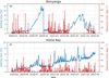 |
Fig. 2 Daily soiling losses (blue solid lines) and rainsum (red dashed lines) observed in Shinyanga (a) and Homa Bay (b). |
2.2 Soiling models
2.2.1 Original HSU model
The original HSU soiling model was developed by Coello and Boyle in order to simulate soiling losses in a simple and accurate way [22]. At each time step, the model considered the particle dry deposition from the atmosphere on the PV module and uses it to estimate the total accumulated particulate mass. Following a similar approach as [17], in this work we assume that the mass deposited on the PV module depends solely on the ambient concentration of particulate matter of diameter below 10 µm (PM10), and a constant value of the deposition velocity vd. On day i, the resulting accumulated mass on the PV module (mi, in g m−2) is calculated by
 (4)
(4)
where i0 refers to the day after the PV module was cleaned by rain or other means for the last time before day i, θ indicates the module's tilt angle, t is the time step between two PM10 data points in seconds, and CT is the considered cleaning threshold. In this work, θ is constant, but the model also allows for considering varying tilt angles. As previously mentioned, the original HSU model considered that, when the daily rain sum surpasses the chosen cleaning threshold, the rain washes away all the mass accumulated up to that day.
Once the time series of total deposited mass over the PV module has been calculated, the corresponding time series of soiling losses is estimated by
 (5)
(5)
where erf indicates the error function.
Both the values of vd and CT need to be optimized to the specific considered location. Values of vd used in the literature range between 0.09 and 0.9 cm s−1 [17,22], and the CT between 1 and 20 mm day−1 [1].
2.2.2 Modified HSU model
The proposed modified HSU model incorporates two novel features into the original HSU model: on one hand, the cleaning effect by precipitation is considered to be a function of the daily rain sum, with which cleaning due to small daily rain sums is also considered, and incomplete cleaning is allowed to happen. On the other hand, a small fraction of the daily deposited mass is considered to permanently adhere to the PV module unless the module is manually cleaned.
The cleaning effect by precipitation is described by the completeness of natural cleaning (CNC). Similar to the approach of [29], the CNC is used to describe the rain's impact on the mass accumulated on the PV module as a logarithmic function of the daily rain sum in mm:
 (6)
(6)
where a and b are the parameters of the logarithmic fit. If the function surpasses a CNC of 0.97, the result is replaced by this value. The logarithmic approach was selected based on statistical superiority as presented in [29] and [14], where alternative functions such as multilinear fits and a random forest approach were also tested.
On a given day, the fraction χ of the mass depositing on the PV module is assumed to permanently adhere. We assume that χ stays constant over the considered period, the total amount of persistent soiling accumulated on a day i (ωi) is given by
 (7)
(7)
The assumption that χ does not change with time is a simplification that excludes several physical effects, such as a seasonal variation of the soiling type and aging of the soiling layer. We select this approach to keep the number of model parameters that have to be calibrated as small as possible.
Taking into consideration both effects described in equations (6) and (8), the daily mass accumulated on the PV panel mi is computed as:
 (8)
(8)
where, similarly to the HSU original case, i0 indicates the day when the last manual cleaning of the PV module was performed, θ indicates the module's tilt angle, t is the considered time step in seconds, and vd is the considered deposition velocity. In order to apply the modified HSU model to a specific location, the parameters a, b, χ, and v_d need to be calibrated for the local conditions (environmental and collector type).
As for the original HSU model, after calculating the daily accumulated mass time series, it is transformed into the corresponding soiling losses following Equation (5).
Although we focus on incomplete cleaning and persistent soiling, we opted for the model formulation without PM2.5. This brings along a limitation, as the finer particles seem to be linked more than coarser particles to rain-resistant soiling [19]. However, it also brings along advantages such as simplicity, a broader application range for data sets without PM2.5, and less model parameters that have to be calibrated. The latter might increase the robustness of the model and avoid overfitting.
2.3 Reanalysis meteorological input
In order to estimate soiling losses, both the original and the modified HSU models need as input data the atmospheric PM10 concentration as well as the daily rain sum. In this work, we employ the Copernicus Atmosphere Monitoring Service (CAMS) global reanalysis EAC4 [30] for daily PM10 concentration and the Copernicus Climate Change Service global reanalysis ERA5 [31] for precipitation. EAC4 and ERA5 are, respectively, the fourth and fifth generations of the European Centre for Medium-Range Weather Forecasts (ECMWF) global reanalysis. Following a principle known as data assimilation, reanalysis data combine a physical-chemical model of the atmosphere with observations from across the world to provide a globally complete and consistent dataset of meteorological variables. Both reanalysis datasets consist of a global grid of 0.25° of resolution in latitude. While ERA5 has the same resolution in longitude (0.25°), the EAC4 grid is coarser and has 0.75° in longitude. In this manuscript, reanalysis data employed to estimate soiling losses corresponding to a specific EAPP station was spatially bilinearly interpolated to the site of interest. Soiling maps were estimated for the coincident PM10 and precipitation data corresponding to the EAC4 grid.
3 Results
3.1 Soiling model calibration
The capabilities of both considered soiling models (HSU original and HSU modified) to reproduce the soiling losses observed at Shinyanga and Homa Bay were tested, for which interpolated EAC4 PM10 concentrations and ERA5 daily rain sums corresponding to the campaign period were used as input data. Then, the parameters that each model relies upon were calibrated to best fit the observations. The calibration was calculated for the period comprehended between the beginning of the campaign (mid-December 2019) and 31st December 2020. This period is called the calibration period hereafter. Calibrating the models using as input ERA5 daily rain sums instead of using the observed precipitation allows to correct a part of the inherent errors present in the reanalysis data for the site of interest. The parameters yielding the best calibration for the specific location characterize the predominant soiling type occurring at the considered site.
The original HSU model was calibrated in order to obtain the values of v_d and CT, yielding simulated soiling losses that minimize the mean root mean square error (RMSE) compared to the observations. The RMSE is defined as
 (9)
(9)
where SLsim,i and SLobs,i indicate the soiling loss simulated and observed, respectively, at each time step, and n indicates the total number of observations.
Two further error metrics are calculated for the modeled soiling losses using the calibrated parameters to further evaluate the calibration results and, later, also for a validation. The bias of the simulated soiling losses is defined as follows:
 (10)
(10)
The mean absolute error (MAE) is defined as
 (11)
(11)
While RMSE rather penalizes large deviations between observations and simulations, MAE shows the average of the absolute differences between observations and simulations, treating all deviations equally. The bias is the average of the signed differences between simulations and observations and assesses whether there is a consistent direction in the deviation: a positive bias indicates overestimation by the simulations, a negative one, otherwise, and a zero bias does not mean a lack of deviation.
Due to the different pattern in the time series of soiling losses observed at Shinyanga and at Homa Bay, the calibration of the modified HSU model follows a different procedure at each station:
For the Shinyanga case, where the soiling losses steadily increase during the dry season and the precipitation is able to remove most of the soiling at the beginning of the rainy season (Fig. 2a), the presence of persistent soiling is unclear. For this reason, we analyzed the minimum soiling losses occurring in the beginning of the rainy season, during the period between 15 November 2020 and 31 December 2020. It was found that the soiling losses never completely reset to 0 but remained at a minimum of 0.13% despite the observed high levels of daily precipitation, pointing toward the existence of a small quantity of non-removable persistent soiling. Assuming this soiling loss was caused only by persistent soiling (i.e., ω, as in Eq. (7)), Equation (5) applied with m = ω revealed a value of ω = 9.6 × 10⁻³ µg m–2 persistently accumulated on top of the PV panel. We also assumed that such an amount of persistent mass would have already been accumulated by the end of the dry period and, hence, would be a fraction of the total mass accumulated (m) by the end of September 2020. The corresponding soiling loss by this date is 11.1%, which, based on Equation (5), indicates a corresponding value of ω = 1.92 × 10⁶ µg m–2. This allows estimating in a first calibration step the expected value for the χ parameter as 0.5%, corresponding to the ratio between the minimum ω estimated for the beginning of the rainy season and the total m estimated for the end of the dry season. This small percentage of daily accumulated persistent soiling χ indicates a type of soiling for this location, which is mostly washable by rain.
Following the determination of χ, vd is subsequently calibrated based on the accumulation of persistent soiling alone. To do so, a time interval of at least two weeks within the calibration period where at least a rain sum of 1 mm day−1 occurred every day is selected. In this case, the entire month of December 2020 was chosen. During this period all non-permanently adhered dirt is supposed to be washed away by rain, and only the persistent soiling is assumed to remain on top of the PV module. The time series of daily accumulated persistent mass is calculated based on Equation (7), and its corresponding soiling losses are derived with Equation (5) adjusted as follows:
 (12)
(12)
The parameters χ is set to the previously derived value of 0.5%, and vd is calibrated to minimize the RMSE between the soiling losses simulated with Equation (12) and the observed soiling losses at Shinyanga during the selected rainy period.
Finally, using the values for χ and vd previously estimated, the parameters a and b are calibrated to minimize the RMSE associated to the soiling losses modelled for the entire calibration period.
In case of the Homa Bay station, where a continuous build-up of the soiling losses is observed, indicating a significant amount of persistent soiling continuously accumulating, the step-wise calibration performed for Shinyanga is not necessary. In this case, the four parameters affecting Equation (8) (χ, vd, a and b) are calibrated simultaneously in order to minimize the RMSE of the soiling losses modelled during the first campaign year.
At both stations, and as for the original HSU model, the calibration is also checked in terms of bias and MAE (Eqs. (10) and (11), respectively).
The calibration results for the parameters corresponding to each model and station are then used to simulate the soiling losses corresponding to the second half of the campaign (from 1st January 2021 to 31st December 2021). This period is denominated validation period, and it shows the performance of the calibrated model. For that purpose, the error metrics given by Equations (9–11) are also calculated for the validation period.
The results corresponding to each considered soiling type are presented in the following sections.
3.1.1 Shinyanga calibration
The calibration of the original HSU model at Shinyanga indicated the lowest RMSE model performance during the calibration period, considering a value of the cleaning threshold of CT = 2.6 mm day−1 and a deposition velocity of vd = 0.009 m s−1. To calibrate the modified HSU model, χ was first set to 0.5%, following the procedure previously explained. Then, the building-up of persistent soiling was characterized for the entire December 2020, yielding a value of vd = 0.011 m s−1. Third, optimal parameter values of a = 0.10 and b = 0.23 were found.
Using these values, the time series of soiling losses predicted by each model for the entire campaign period was produced. The comparison of the predicted soiling losses with the observations is shown in Figure 3. During the calibration period, both HSU model options roughly follow the observations. Both models underestimate the SL in the first months. In the dry season of the calibration period, the modified HSU model first overestimates the SL by up to about 1% and then underestimates the soiling loss after a rain event with a small rain sum below the original HSU model's threshold. The original HSU model follows the observation more closely in the dry season but underestimates SL after a rain event at the end of September 2020. After this rain event the HSU modified model produces an incomplete cleaning event and overestimates SL for about two weeks by about 1%. After the first strong rainfall of the rainy season the HSU original model underestimates the SL stronger than the modified version.
The error metrics for the calibration period are shown in Table 1. The HSU original model performs better than the HSU modified one in terms of RMSE and MAE for this period. The modified HSU model achieves a smaller absolute bias. Both model options show a negative bias.
The situation is different during the validation period. In this case, the partial cleaning effect featured by the modified HSU model helps it to reproduce the observations in a more accurate way than the original HSU model: as the latter considers a complete cleaning of the PV modules every time the daily rain sum surpasses 2.6 mm, this applies also for a small rain event in July 2021. The complete cleanings by rain caused the original HSU model to strongly underestimate the observations for great parts of the validation period. The better performance of the modified HSU model during the validation period is also reflected in the error metrics in Table 1.
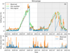 |
Fig. 3 (a) Model optimization for the mostly removable soiling type observed at the Shinyanga station. The blue line shows the time series of soiling losses produced with the calibrated original HSU model, whereas the green line corresponds to the modified HSU model. While the training period is indicated with a white background and solid lines in panel (a), the shaded background and dashed lines correspond to the validation period. The observed soiling losses at Shinyanga are depicted by the solid orange line across the entire campaign period. Panel (b) shows the observed daily rain sum (orange line) at the station, as well as the corresponding ERA5 values (blue line). |
Error metrics and calibration results for the original and modified HSU models calibrated for the soiling conditions observed during the first year at Shinyanga.
3.1.2 Homa Bay calibration
During the calibration period, the best performance of the original HSU model was found for a cleaning threshold of 18.5 mm day−1 and a deposition velocity of 0.0007 m s−1. While the calibration of CT for Homa Bay displays a much higher value than that of Shinyanga (2.6 mm day−1), the particles at Homa Bay are assumed to deposit on top of the PV panels with a lower deposition velocity than at Shinyanga (0.009 m s−1).
In the case of the modified HSU model, the calibration's first step yielded a deposition velocity of vd = 0.007 m s−1, which indicates a slower deposition of the pollutants on top of the PV panels than at Shinyanga (similar to the case of the original HSU model) and a daily percentage of accumulated persistent soiling of χ = 2.5% , significantly higher than the one estimated for Shinyanga (χ = 0.5%). Secondly, the calibration yielded values of a = 0.3 and b = 0.08, showing a cleaning effect by rain larger than the one estimated for Shinyanga (a = 0.10 and b = 0.23).
The comparison between observed and predicted soiling losses at Homa Bay is shown in Figure 4. In this case, the original HSU model is unable to reproduce the continuous increase of the soiling losses observed at this station, produced by the continuous accumulation of firmly adherent mass, which cannot be removed by the rain. Hence, the HSU model underestimates the soiling losses during most of the campaign period, impacting the error metrics shown in Table 2. The best calibration result for the cleaning threshold is very high (18.5 mm day−1), so that at least at times a missed partial cleaning for which the model assumes no cleaning at all occurs, which compensates for the frequent overestimation of cleaning for very strong rain above the cleaning threshold. For a soiling type with the characteristics observed at Homa Bay, the original HSU model performs significantly worse than the modified HSU model in terms of bias, RMSE, and MAE during both the calibration and the validation period.
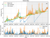 |
Fig. 4 (a) Model optimization for the soiling type observed at the Homa Bay station, where a significant amount of persistent soiling is present. The blue and green lines show the time series of soiling losses produced by the calibrated original and modified HSU models, respectively. The background in panel (a) indicates the calibration period, while the validation period is denoted by the shaded background, along with the dashed lines. The observed soiling losses at Homa Bay are depicted by the solid orange line across the entire campaign period. Panel (b) shows the observed daily rain sum (orange line) at the station, as well as the corresponding ERA5 values (blue line). |
Error metrics and calibration results for the original and modified HSU models calibrated for the soiling conditions observed in the first year at Homa Bay.
3.2 Soiling maps
The calibrated parameters for the locations of Shinyanga and Homa Bay characterize the properties of the soiling type predominant at each station during 2020. Assuming that the properties of the soiling type remain unchanged during long periods of time, the previously introduced soiling models (HSU original and modified) are used to estimate the soiling losses expected for long-term periods of time corresponding to each soiling type. Hence, the average expected soiling losses without manual cleaning for a 20-yr operation period are estimated. The 20 yr were selected as an example of the depreciation time of a PV plant.
Using as input for the soiling models 2D reanalysis gridded data allows estimating the long-term soiling losses at different locations than the calibration sites and, hence, producing maps of long-term trends of soiling losses. This assumes that the presence of a uniform kind of soiling, similar to that occurring at the calibration site, affects the complete considered geographical map. This strongly affects the way in which the maps are intended to be used: the idea is not to create one single map valid for all possible use cases but to provide example maps corresponding to different types of soiling. If the user expects the soiling type of one particular map to occur at their site(s) of interest, that corresponding map can be used. If the user does not know the soiling type or considers various soiling types as possible, various soiling maps should be consulted to estimate the soiling losses for the sites of interest.
The maps permit estimating the 2D spatial variability of the uncertainty associated with two effects: on the one hand, the neglect of the incomplete cleaning effects considered by the modified HSU model (i.e., incomplete cleaning by rain and the presence of persistent soiling), and on the second hand, the error associated with the unknown soiling type affecting each location.
Following this approach, maps representing the geographical distribution of the soiling losses in Europe are created featuring the average soiling losses for the period between 2003 and 2023 (corresponding to the available EAC4 and ERA5 reanalysis input data, shown in Fig. A2). Such maps are produced with both the original and modified HSU models and for the soiling types observed at Shinyanga and Homa Bay. In order to cover such a large geographical area as the European continent, the considered tilt angle in the simulations was adjusted to a value rather close to its optimal value for PV production for selected locations within three different latitude bands. For determining the optimal tilt angle, the Global Solar Atlas was used (https://globalsolaratlas.info/map). In this way, southern European latitudes between 30°N and 45°N consider a tilt angle of θ = 35°, central European latitudes between 45°N and 55°N consider a tilt angle of θ = 39°, and northern European latitudes between 55° and 80° consider a tilt angle of θ = 45°. This has been done to remove a possible systematic effect of the tilt angle for the maps at least partly. The corresponding maps are shown in the following sections.
3.2.1 Removable soiling type (Shinyanga calibration)
The European maps showing the average soiling loss estimated for the period between 2003 and 2023 estimated using the calibrations corresponding to the soiling type observed at Shinyanga during 2020 are shown in Figure 5. Both maps show the cleaning effect of the frequent, abundant precipitation in northern European regions, displaying low values of the soiling losses in this region. On the other hand, various big cities and highly industrialized areas, such as the Po region (northern Italy), display high soiling losses independently of the used approach.
While the map corresponding to the original HSU model produces average soiling losses up to a maximum of 2%, the incomplete cleaning effects incorporated into the modified HSU model take this maximum up to 5%. This characterizes the order of magnitude of the underestimation expected for this soiling type when long-term trends of soiling losses are estimated with the original HSU model in comparison to the estimations of the modified HSU version. This underestimation was expectable, as the model showed a strong negative bias for the validation phase in Shinyanga (Fig. 3a). The underestimation by the original HSU model is also apparent on the average soiling loss estimated for the entire European continent as well as for the German and Andalusian (southern Spain) regions, representative, respectively, of the central- and southern European areas (Tab. 3). For the entire continent, soiling loss estimates with the HSU model are 4 times lower than the ones estimated with the modified HSU model. However, this underestimation is not homogeneous: in the German case, the underestimation reaches approximately a factor of 1/5, whereas in the Andalusian case, it is only about 1/2.
Besides, Figure 5 and Table 3 also show that considering the Shinyanga type of soiling, mostly washable away by rain, results in a north-to-south increasing trend over the European continent, as displayed by both models. While soiling losses estimated with the original HSU model are on average 3.4 times larger in Andalusia than in Germany, this difference is smaller when estimated with the modified HSU model, with the Andalusian losses being on average only 1.3 times larger than the German ones.
 |
Fig. 5 Maps of average soiling losses in Europe for PV operation without manual cleaning over 20 yr (2003–2023) using the original HSU model (a) and its modified version (b) with the corresponding parameters calibrated for the soiling type observed in Shinyanga during 2020 (see Tab. 3). The color bar limits are different for the two cases: Due to the different magnitude of the estimated soiling losses by each model, the color bar in panel (a) reaches up to 2%, whereas the color bar in panel (b) reaches up to 5%. |
Average long-term soiling loss for PV operation without manual cleaning over 20 yr (2003–2023) for specific regions in Europe was estimated with both the original and the modified HSU soiling models for the calibration corresponding to the soiling type observed in Shinyanga during 2020. Ranges (max.–min.) are shown in brackets. The calibration results are also provided in the table header.
3.2.2 Persistent soiling type (Homa Bay calibration)
Figure 6 shows the European maps displaying the average soiling loss without manual cleaning for the period 2003–2023, estimated using the calibration characterizing the soiling conditions at Homa Bay in 2020. Despite consisting of a larger fraction of persistent material than the soiling present at Shinyanga, the maps in Figure 6 present similarities to those in Figure 5: the northernmost European region is the region less affected by soiling losses, thanks to the abundant and frequent precipitation. The high concentrations of particulate matter around several bigger cities and in the Po region are also present in Figure 6b (HSU modified). The soiling map produced with the original HSU model is dominated by the exceptionally high cleaning threshold of 18.3 mm day-1 (see Fig. 1A). In this approach, frequent precipitation is not sufficient to clean the PV modules; it must also be exceptionally abundant. This leads to relatively high levels of soiling in regions such as Germany.
Similarly to the Shinyanga case, the original HSU model underestimates the soiling losses. However, in this case, the underestimation, and hence the error due to neglecting the persistent soiling, is larger: at the European level, HSU original estimates maximum soiling losses of 2%, compared to the maximum 10% indicated by the modified HSU model. This can also be observed at the corresponding European, German, and Andalusian averages, displayed in Table 4: on average, neglecting the significant fraction of highly adherent pollutants included in this soiling type would lead to an underestimation of 5.6 times compared to the soiling losses produced with the modified HSU model. For Germany, this underestimation is reduced to 4.9 times, and for Andalusia to 5.3 times.
Compared to the Shinyanga soiling type, the higher fraction of persistent soiling produces long-term soiling losses that are about twice as large. Additionally, the north-to-south variability observed when considering a soiling type mainly removable by rain is erased when considering the Homa Bay soiling type. In this case, independently of the used model, the soiling losses estimated for Germany slightly surpass the soiling losses estimated for Andalusia, as can be observed in Table 4.
 |
Fig. 6 Maps of averaged soiling losses in Europe for PV operation without manual cleaning over 20 yr (2003–2023) using the original HSU model (a) and its modified version (b) with the corresponding parameters calibrated for the soiling type observed in Homa Bay during 2020 (see Tab. 4). The color bar limits are different for the two cases and, in the case of the modified model, also different from the map based on the Shinyanga calibration. Due to the different magnitude of the estimated soiling losses by each model, the color bar in panel (a) reaches up to 2%, whereas the color bar in panel (b) reaches up to 10%. |
Average long-term soiling loss for PV operation without manual cleaning over 20 yr (2003–2023) for specific regions in Europe was estimated with both the original and the modified HSU soiling models for the calibration corresponding to the soiling type observed at Homa Bay during 2020. Ranges (max.–min.) are shown in brackets. The calibration results are also provided in the header.
3.2.3 Discussion of uncertainty and comparison of the maps with results from literature
The uncertainty of the data shown in the maps is influenced by various factors. Based on the strong deviations of the maps for each of the two evaluated model types caused by the two different calibrations, one can expect that the knowledge of the soiling type is a main uncertainty driver. If the user of an exemplary map does not know that the soiling type and input data errors present at the site(s) of interest are the same as for the example map, the results shown in the map for these sites can deviate strongly from the actual soiling losses. For the average for Germany in our example maps, a factor 2.5 was caused by changing between the two soiling types for both the original and the modified model. If the soiling type is known and if input data errors are reduced by the site-specific calibration, the uncertainty is lower but still significant. The minimum of the uncertainties for this case can be estimated using the RMSE of the validation data sets evaluated in Homa Bay and Shinyanga for sites with a similar average soiling loss (Tabs. 1 and 2). Those RMSEs must be combined with the uncertainty of the reference soiling measurements, which is about 1% for measurements with PV device pairs [14]. This corresponds to a minimum uncertainty of 1.5% for the modified model and 2.3% for the original model in the first two years after a manual cleaning. For sites with frequent and abundant rain and low PM10 the uncertainties are lower than for sites with high PM10 and/or low and infrequent rain. For longer periods without cleaning, the uncertainty grows due to the uncertainty of χ. This also leads to the recommendation to plan periodic cleanings at least every couple of years even in rainy areas to reduce the uncertainty of yield estimations and the risk of production losses.
An additional uncertainty influence stems from soiling types that are excluded from the model because they are not driven by the PM10 and because they did not appear in the underlying ground measurements (e.g., lichen, moss, and other biological growths). Bird droppings are only partly included in the data, as the reference cells are small and as extreme soiling values caused by bird droppings can lead to the exclusion of the data in the processing routine. Depending on the site, these soiling types can lead to high additional soiling losses that are not considered in our model. Hence, for cases with such soiling types, our model would underestimate the soiling losses.
We compared the results to long-term soiling data in the form of maps and long-term soiling experiments from selected publications. A perfect match of the experimental findings from the literature and the 20-yr average losses of our maps cannot be expected, not only because of the model and input data uncertainty but also because of the fact that we only investigate two specific soiling types. However, the comparison can help to check if the results are reasonable, and it increases the understanding of the results.
In a first step our maps with the original HSU model were compared to those with the original HSU model from [17]. For the Shinyanga calibration the maps closely match. With the Homa Bay calibration, significant differences are found as expected due to the high cleaning threshold in our calibration.
The comparison of the long-term experimental soiling from rainy sites is of particular interest for our study. In [17], a 2.53% per year soiling rate was derived for Burgdorf, Switzerland, based on [9]. This would lead to approximately 25.3% average 20-yr soiling loss. This is much higher than the about 5% found in our case for the site with the persistent soiling type from Homa Bay. Such a deviation is, however, not a contradiction but possible, as it is clear that the soiling type used in our maps can deviate from the case in Burgdorf. It was mentioned in [17] that brake dust might be a main contributor to the soiling losses in Burgdorf, and hence, lower losses and better rain cleaning for the two soiling types from our study seem reasonable.
In [18], manual cleaning of PV modules after more than 7 yr without cleaning caused a 5 to 11% performance increase for five investigated sites in North Carolina (USA). This interval of observed losses fits the range of soiling losses in our maps with the modified HSU model based on the Homa Bay calibration. This indicates that the soiling types in [18] can be considered to be persistent.
Lopez-Garcia et al. [8] found an average annual soiling rate of 0.31% per year in their over 30-yr-long data set of PV modules without any cleaning in Ispra, Italy. For the 20-yr average, this would correspond to approximately 3.1% average losses. This is slightly lower than the about 5% losses found for Ispra in our results with the modified model and the Shinyanga calibration. The deviation is considered to be small given the likely difference in soiling types and to be even within the model's uncertainties. A deviation can also be caused due to the different and, in our case, shorter time interval.
The maps from the original HSU model underestimate the soiling losses in comparison to the three described field data sets from the literature. They are therefore considered to be unrealistic for long-term soiling estimation and to strongly underestimate the soiling losses even for many rainy sites. The modified HSU model with the two soiling types used for the maps results in average soiling losses within the range of the three experimental studies, which is encouraging.
4 Summary and conclusion
In order for soiling models to produce realistic estimates of long-term soiling losses, the incomplete cleaning effect of rain, as well as the potential presence of a certain fraction of highly adherent pollutants among the accumulated soiling, needs to be considered.
In this study, we analyze the natural variability of the soiling losses observed at two EAPP stations (Shinyanga and Homa Bay) during a two-year campaign, with one reference cell that was not manually cleaned. The only cleaning effects were, therefore, due to the natural processes and, in particular, the rainfall. At both stations, incomplete cleaning by rain, when the soiling losses were not reset to 0, was observed. However, while at Shinyanga the rain was able to effectively remove most of the pollution accumulated on the reference cell, at Homa Bay, the soiling losses kept steadily increasing despite the abundant levels of precipitation constantly observed during the campaign period. This points toward the presence of a larger fraction of sticky material in Homa Bay.
Elaborating on the work of [14] based on these observations, we modified the original HSU model to incorporate not only the incomplete cleaning effect by rain but also the assumption that a certain fraction of the mass that accumulates daily on the PV module adheres permanently and cannot be removed by rain. Thereafter, both model versions were calibrated to the Shinyanga and Homa Bay soiling types, considering the first year of observations. The calibration results for the parameters of the original model deviate noticeably from default values from the literature and indicate the high importance of a site-specific calibration. The calibrated models were then used to estimate the soiling losses observed during the second campaign year. The error metrics for the validation showed the improved performance of the modified HSU model with respect to the original version.
Soiling models applied to gridded input data have the capability of producing maps of the 2D geographical variability of the soiling losses, as it was shown by Fernández Solas et al. [17]. Similarly, we used 20 yr of trends of input parameters to estimate the long-term variability of the soiling losses in Europe, considering the two soiling types corresponding to Shinyanga and Homa Bay. The application of model parameters derived for the African sites for Europe is considered to be valid for the demonstration of the method and delivers exemplary results that might also occur for soiling types found at some European sites. Each map represents the soiling losses for a specific exemplary soiling type with a given rain cleaning effect. The derived different soiling maps are examples of soiling types that might be found at some European sites. The maps hence demonstrate the method and illustrate the magnitude of soiling losses that have to be expected for different soiling types. The maps should, however, not be understood as the most likely possible values for European soiling. For both soiling types, it was found that employing the original HSU model would yield significant underestimations of the soiling losses, highlighting the importance of the newly incorporated effects. The discrepancies found between the maps corresponding to both soiling types (with the soiling losses corresponding to Homa Bay being about twice the ones corresponding to Shinyanga) illustrate the uncertainty existing at the European level due to the typically unknown soiling types. Depending on the considered soiling type, the north-to-south variability of the soiling losses can be more or less pronounced, and, in cases with a significant amount of persistent soiling, Germany can reach similar soiling losses to the ones estimated for Andalusia.
The method used to create the soiling maps should be further evaluated and validated with more data from various sites and climates in future studies. The method can also be applied to test the effect of different manual cleaning frequencies and decide on the optimal cleaning schedules. Further improvements of the soiling models and a full characterization of the soiling particles would be of interest for such improvements. For example, the current model does not consider, e.g., seasonal variations of the soiling type, aging of the soiling layer, lichens, moss, and other biological growths. Additionally, bird droppings were, at least partly, excluded from the data processing. To include these effects, the so far constant model parameters a, b, vd, and χ would have to change with time, and it is likely that PM-independent terms would have to be added.
The European maps presented in this study can be used by stakeholders in the PV community for several purposes: besides describing the uncertainty associated with long-term trends of soiling losses estimated at the European level due to the unknown soiling type, they can also be helpful to estimate the soiling losses for PV yield analysis at different locations, especially in feasibility studies. Additionally, the provided information on the soiling conditions can help to decide on the most appropriate mitigation measures.
Acknowledgments
The authors would like to thank GeoSUN Africa, the World Bank, the East African Power Pool, and the EAPP station responsible for providing the data used in this study. We also thank the European Centre for Medium-Range Weather Forecast (ECMWF), the Copernicus Atmosphere Monitoring Service (CAMS), and the Copernicus Climate Change Service for providing the reanalysis meteorological data used in our work.
We would also like to thank Laura Campos Guzmán for sharing the software to process soiling losses and her technical support. We thank Anne Forstinger for the insightful conversation that pointed us toward the data used in this study. Finally, we thank the reviewers for their helpful comments.
Funding
We thank the European Union for funding the CAMEO project (grant agreement 101082125).
Conflicts of interest
The authors declare no conflict of interest.
Data availability statement
The data that support the findings of this study are available from the corresponding author upon reasonable request.
Author contribution statement
E.R.D. led the conceptualization, methodology, software, validation, formal analysis, investigation, resources, data curation, visualization, and writing—original draft preparation; F.N.S. supported the conceptualization, methodology, validation, formal analysis, investigation, and writing—review and editing; A.F.S. supported the conceptualization, methodology, validation, formal analysis, investigation, and writing—review and editing; N.H. supported the conceptualization, methodology, investigation, writing—review and editing, and funding acquisition; L.M. supported the conceptualization, methodology, investigations, and writing—review and editing; J.A.M. supported the methodology, investigations, and writing—review and editing; J.P. supported the methodology, investigations, and writing—review and editing; L.Z. supported the methodology, investigations, and writing—review and editing; S.W. supported the conceptualization, methodology, validation, formal analysis, investigation, resources, visualization, writing—review, revision, and editing, and led the supervision and funding acquisition.
References
- K. Ilse, L. Micheli, B. Figgis, K. Lange, D. Daßler, D.H. Hanifi, F. Wolfertstetter, V. Naumann, C. Hagendorf, R. Gottschalg, J. Bagdahn, Techno-economic assessment of soiling losses and mitigation strategies for solar power generation, Joule 3, 2303 (2019). https://doi.org/10.1016/j.joule.2019.08.019 [Google Scholar]
- W. Jo, N. Ham, J. Kim, J. Kim, The cleaning effect of photovoltaic modules according to precipitation in the operation stage of a large-scale solar power plant, Energies 16, 6180 (2023). https://doi.org/10.3390/en16176180 [Google Scholar]
- M. Redondo, C.A. Platero, A. Moset, F. Rodríguez, V. Donate, Soiling modelling in large grid-connected PV plants for cleaning optimization, Energies 16, 904 (2023). https://doi.org/10.3390/en16020904 [Google Scholar]
- L. Micheli, E.F. Fernández, J.T. Aguilera, F. Almonacid, Economics of seasonal photovoltaic soiling and cleaning optimization scenarios, Energy 215, 119018 (2021). https://doi.org/10.1016/j.energy.2020.119018 [Google Scholar]
- L. Micheli, E.F. Fernández, F. Almonacid, Photovoltaic cleaning optimization through the analysis of historical time series of environmental parameters, Sol. Energy 227, 645 (2021). https://doi.org/10.1016/j.solener.2021.08.081 [Google Scholar]
- L. Micheli, E.F. Fernández, M. Muller, F. Almonacid, Extracting and generating PV soiling profiles for analysis, forecasting, and cleaning optimization, IEEE J. Photovolt. 10, 197 (2020). https://doi.org/10.1109/JPHOTOV.2019. 2943706 [Google Scholar]
- P. Besson, C. Muñoz, G. Ramírez-Sagner, M. Salgado, R. Escobar, W. Platzer, Long-term soiling analysis for three photovoltaic technologies in Santiago region, IEEE J. Photovolt. 7, 1755 (2017). https://doi.org/10.1109/JPHOTOV.2017.2751752 [Google Scholar]
- J. Lopez-Garcia, A. Pozza, T. Sample, Long-term soiling of silicon PV modules in a moderate subtropical climate, Sol. Energy 130, 174 (2016). https://doi.org/10.1016/j.solener.2016.02.025 [Google Scholar]
- C. Schill, A. Anderson, C. Baldus-Jeursen, L. Burnham, L. Micheli, D. Parlevliet, E. Pilat, B. Stridh, E. Urreloja, M. Basappa Ayanna, G. Cattaneo, S.J. Ernst, A. Kottantharayil, G. Mathiak, E. Whitney, R. Neukomm, D. Petri, L. Pratt, L. Rustam, T. Schott, Soiling losses—impact on the performance of photovoltaic power plants report IEA-PVPS T13-21:2022 (2022). https://iea-pvps.org/key-topics/soiling-losses-impact-on-the-performance-of-photovoltaic-power-plants/ [Google Scholar]
- J.G. Bessa, L. Micheli, J. Montes-Romero, F. Almonacid, E.F. Fernández, Estimation of photovoltaic soiling using environmental parameters: a comparative analysis of existing models, Adv. Sustainable Syst. 6, 2100335 (2022). https://doi.org/10.1002/adsu.202100335 [Google Scholar]
- J. Lopez-Lorente, J. Polo, N. Martín-Chivelet, M. Norton, A. Livera, G. Makrides, G.E. Georghiou, Characterizing soiling losses for photovoltaic systems in dry climates: a case study in Cyprus, Sol. Energy 255, 243 (2023). https://doi.org/10.1016/j.solener.2023.03.034 [Google Scholar]
- N. Hanrieder, S. Wilbert, F. Wolfertstetter, J. Polo, C. Alonso, L. Zarzalejo, Why natural cleaning of solar collectors cannot be described using simple rain sum thresholds, Proc. ISES Sol. World Congr. (2021). https://www.swc2021.org/ [Google Scholar]
- M. Valerino, M. Bergin, C. Ghoroi, A. Ratnaparkhi, G.P. Smestad, Low-cost sol. PV soiling sensor validation and size resolved soiling impacts: a comprehensive field study in Western India, Sol. Energy 204, 307 (2020). https://doi.org/10.1016/j.solener.2020.03.118 [Google Scholar]
- F. Norde Santos, S. Wilbert, E. Ruiz Donoso, J. El Dik, L. Campos Guzman, N. Hanrieder, A. Fernández García, C. Alonso García, J. Polo, A. Forstinger, R. Affolter, R. Pitz-Paal, Cleaning of photovoltaic modules through rain: experimental study and modeling approaches, Sol. RRL 8, 2400551 (2024). https://doi.org/10.1002/solr.202400551 [Google Scholar]
- S. You, Y. Jie Lim, Y. Dai, C.-H. Wang, On the temporal modelling of solar photovoltaic soiling: energy and economic impacts in seven cities, Appl. Energy 228, 1136 (2018). https://doi.org/10.1016/j.apenergy.2018.07.020 [Google Scholar]
- X. Li, D.L. Mauzerall, M.H. Bergin, Global reduction of solar power generation efficiency due to aerosols and panel soiling, Nat. Sustain. 3, 720 (2020). https://doi.org/10.1038/s41893-020-0553-2 [Google Scholar]
- A. Fernández Solas, N. Riedel-Lyngskær, N. Hanrieder, F. Norde Santos, S. Wilbert, H. Nygard Riise, J. Polo, E.F. Fernández, F. Almonacid, D.L. Talavera, L. Micheli, Photovoltaic soiling loss in Europe: geographical distribution and cleaning recommendations, Renew. Energy 239, 122086 (2025). https://doi.org/10.1016/j.renene.2024. 122086 [Google Scholar]
- J.G. Bessa, M. Valerino, M. Muller, M. Bergin, L. Micheli, F. Almonacid, E. Fernandez, An Investigation on the Pollen-Induced Soiling Losses in Utility-Scale PV Plants, in 2023 IEEE 50th Photovoltaic Specialists Conference (PVSC) (San Juan, Puerto Rico, 2023). https://doi.org/10.1109/PVSC48320.2023.10359930 [Google Scholar]
- S. Toth, M. Hannigan, M. Vance, M. Deceglie, Predicting photovoltaic soiling from air quality measurements, IEEE J. Photovolt. 10, 1142 (2020). https://doi.org/10.1109/JPHOTOV.2020.2983990 [Google Scholar]
- D. Kumar, K. Ritter, J. Raush, F. Ferdowsi, R. Gottumukkala, T. Chambers, Optimizing photovoltaic soiling loss predictions in Louisiana: a comparative study of measured and modeled data using a novel approach, Prog. Photovolt. Res. Appl. 33, 560 (2025). https://doi.org/10.1002/pip.3891 [Google Scholar]
- L. Micheli, G.P. Smestad, J.G. Bessa, M. Muller, E.F. Fernández, F. Almonacid, Tracking soiling losses: assessment, uncertainty, and challenges in mapping, IEEE J. Photovolt. 12, 114 (2022). https://doi.org/10.1109/JPHOTOV.2021.3113858 [Google Scholar]
- M. Coello, L. Boyle, Simple model for predicting time series soiling of photovoltaic panels, IEEE J. Photovolt. 9, 1382 (2019). https://doi.org/10.1109/JPHOTOV.2019. 2919628 [Google Scholar]
- Energydata.info: https://energydata.info/dataset/?q=geosun&sort=score+desc%2C+metadata_modified+desc (Last accessed 29/09/2025) [Google Scholar]
- J. Peterson, J. Chard, J. Robinson, Extraction of prevailing soiling rates from soiling measurement data, in IEEE 49th Photovoltaics Specialists Conference (PVSC) (Philadelphia, PA, USA, 2022), pp. 0684–0691. https://doi.org/10.1109/PVSC48317.2022.9938838. [Google Scholar]
- Orytech (Pty) Ltd., Homa Bay OR19-16 test site—atmospheric corrosivity (first and second year), report, 2022a. https://energydata.info/dataset/8f50218b-43af-4352-a317-2e333659f2b4/resource/964691b3-c4e3-4856-81cb-2d244d2e593a/download/homa-bay-or19-16-test-site-corrosion-monitoring-data-2-years.pdf (last accessed 12 March 2026) [Google Scholar]
- Orytech (Pty) Ltd., Shinyanga OR19-9 test site—atmospheric corrosivity (first and second year), report, 2022b. https://energydata.info/dataset/ef9491e5-209e-48f7-b6cc-aff6f1565bb0/resource/5fa35e7f-ebfd-4825-8563-b2907013fbf8/download/shinyanga-or19-9-test-site-corrosion-monitoring-data-2-years.pdf (last accessed 12 March 2026) [Google Scholar]
- A. Avila, I. Queralt-Mitjans, M. Alarcón, Mineralogical composition of African dust delivered by red rains over northeastern Spain, J. Geophys. Res. 102, 21977 (1997). https://doi.org/10.1029/97JD00485 [Google Scholar]
- G. Louis, A.S. Kumar, The red rain phenomenon of Kerala and its possible extraterrestrial origin, Astrophys. Space Sci. 302, 175 (2006). https://doi.org/10.1007/s10509-005-9025-4 [Google Scholar]
- F. Norde Santos, S. Wilbert, C. Becker, E. Ruiz-Donoso, L. Campos Guzmán, A. Fernández Solas, L. Zarzalejo, A. Forstinger, D. Helten, V. Pietsch, R. Pitz-Paal, Soiling forecasts for cleaning schedule optimization (poster presentation), European Photovoltaic Solar Energy Conference and Exhibition (EUPVSEC) (2025, Bilbao, Spain, 2025) [Google Scholar]
- A. Inness, M. Ades, A. Agustí-Panareda, J. Barré, A. Benedictow, A.-M. Blechschmidt, J.J. Dominguez, R. Engelen, H. Eskes, J. Flemming, V. Huijnen, L. Jones, Z. Kipling, S. Massart, M. Parrington, V.-H. Peuch, M. Razinger, S. Remy, M. Schulz, M. Suttie, The CAMS reanalysis of atmospheric composition, Atmos. Chem. Phys. 19, 3515 (2019). https://doi.org/10.5194/acp-19-3515-2019 [Google Scholar]
- H. Hersbach, B. Bell, P. Berrisford et al., The ERA5 global reanalysis, Q.J.R. Meteorol. Soc. 146, 1999 (2020). https://doi.org/10.1002/qj.3803 [Google Scholar]
Cite this article as: Elena Ruiz-Donoso, Fernanda Norde Santos, Álvaro Fernández Solas, Natalie Hanrieder, Leonardo Micheli, Joaquín Alonso-Montesinos, Jesus Polo, Luis Zarzalejo, Stefan Wilbert, Maps of long-term soiling losses in Europe considering a partial cleaning effect by rain, EPJ Photovoltaics 17, 17 (2026), https://doi.org/10.1051/epjpv/2026010
Appendix
Due to the uniqueness of the soiling losses observed at Homa Bay by the never-manually-cleaned reference cell, displaying a continuous build-up throughout the campaign period despite the continuous, frequent rainfall, the soiling losses recorded by the monthly manually cleaned reference cell were also analyzed. We aimed to confirm that the signature observed by the never-manually cleaned reference cell was indeed due to the accumulation of soiling and discard possible instrumental malfunctioning. The results are presented in Figure A1. During the one-month intervals between manual cleanings, significant soiling losses, above 2% in many cases, were observed. These soiling losses occurred despite the abundant precipitation at Homa Bay's location and hence confirm the physical plausibility of the observations by the never-manually cleaned reference cell.
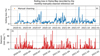 |
Fig. A1 Soiling losses observed by the monthly manually cleaned reference cell in Homa Bay (a), with the manual cleaning dates indicated by the orange dots. The station precipitation, in terms of daily rain sum, is displayed on panel (b). |
The soiling maps presented in Section 3.2 use as input 20 years of PM10 concentrations from EAC4 reanalysis and daily rain sums from ERA5 reanalysis. Hence, the resulting 2D distribution of the time-averaged soiling losses is affected by the 2D distribution of the input parameters, shown in Figure A2a (PM10) and A2b (rain sum). The PM10 concentrations strongly depend on the local sources of particles, with highly industrialized areas, as well as capital cities, displaying the maximum daily levels on average.
 |
Fig. A2 European map showing the average values for the period between 2003 and 2023 for EAC4 average PM10 concentrations (a) and ERA5 daily rain sums (b). The number of days within the considered 20-year period when the ERA5 daily rain sum estimated for each location surpassed the cleaning threshold of 18.35 mm day-1 are presented on panel (c). |
The precipitation presents, on average, its maximum daily levels in northern and mountainous regions and its minimum values in southern regions. The trade-off between the accumulation of particles and the rain cleaning determines the soiling patterns observed in Figure 3a (map derived with the original HSU model and the Shinyanga soiling type), Figure 3b (map derived with the modified HSU model and the Shinyanga soiling type), and Figure 4b (map derived with the modified HSU model and Homa Bay soiling type). Besides the input data, the 2D soiling distribution generated by the calibrated original HSU model for the Homa Bay soiling type, shown in Figure 4a, is determined by the unusually high cleaning threshold of 18.35 mm day-1. With this condition, in order for PV panels to be cleaned by rain, the latter needs to be not only frequent but extremely abundant. Figure A2c shows the number of days in the period 2003–2023 when the daily rain sum at each location in Europe surpassed such a threshold. The regions showing a scarce occurrence of this condition coincide with those presenting larger soiling losses in Figure 4a.
All Tables
Error metrics and calibration results for the original and modified HSU models calibrated for the soiling conditions observed during the first year at Shinyanga.
Error metrics and calibration results for the original and modified HSU models calibrated for the soiling conditions observed in the first year at Homa Bay.
Average long-term soiling loss for PV operation without manual cleaning over 20 yr (2003–2023) for specific regions in Europe was estimated with both the original and the modified HSU soiling models for the calibration corresponding to the soiling type observed in Shinyanga during 2020. Ranges (max.–min.) are shown in brackets. The calibration results are also provided in the table header.
Average long-term soiling loss for PV operation without manual cleaning over 20 yr (2003–2023) for specific regions in Europe was estimated with both the original and the modified HSU soiling models for the calibration corresponding to the soiling type observed at Homa Bay during 2020. Ranges (max.–min.) are shown in brackets. The calibration results are also provided in the header.
All Figures
|
Fig. 1 Locations of the EAPP stations in Kenya, Uganda, and Tanzania, with the stations used in this study (Shinyanga and Homa Bay) highlighted in green (a). Measurement station at Homa Bay (b) and zoom into the three reference cells used to estimate soiling losses (c). Image sources: (a) Google Earth; (b) and (c) Homa Bay station information report by GeoSUN [23]. |
| In the text | |
|
Fig. 2 Daily soiling losses (blue solid lines) and rainsum (red dashed lines) observed in Shinyanga (a) and Homa Bay (b). |
| In the text | |
|
Fig. 3 (a) Model optimization for the mostly removable soiling type observed at the Shinyanga station. The blue line shows the time series of soiling losses produced with the calibrated original HSU model, whereas the green line corresponds to the modified HSU model. While the training period is indicated with a white background and solid lines in panel (a), the shaded background and dashed lines correspond to the validation period. The observed soiling losses at Shinyanga are depicted by the solid orange line across the entire campaign period. Panel (b) shows the observed daily rain sum (orange line) at the station, as well as the corresponding ERA5 values (blue line). |
| In the text | |
|
Fig. 4 (a) Model optimization for the soiling type observed at the Homa Bay station, where a significant amount of persistent soiling is present. The blue and green lines show the time series of soiling losses produced by the calibrated original and modified HSU models, respectively. The background in panel (a) indicates the calibration period, while the validation period is denoted by the shaded background, along with the dashed lines. The observed soiling losses at Homa Bay are depicted by the solid orange line across the entire campaign period. Panel (b) shows the observed daily rain sum (orange line) at the station, as well as the corresponding ERA5 values (blue line). |
| In the text | |
|
Fig. 5 Maps of average soiling losses in Europe for PV operation without manual cleaning over 20 yr (2003–2023) using the original HSU model (a) and its modified version (b) with the corresponding parameters calibrated for the soiling type observed in Shinyanga during 2020 (see Tab. 3). The color bar limits are different for the two cases: Due to the different magnitude of the estimated soiling losses by each model, the color bar in panel (a) reaches up to 2%, whereas the color bar in panel (b) reaches up to 5%. |
| In the text | |
|
Fig. 6 Maps of averaged soiling losses in Europe for PV operation without manual cleaning over 20 yr (2003–2023) using the original HSU model (a) and its modified version (b) with the corresponding parameters calibrated for the soiling type observed in Homa Bay during 2020 (see Tab. 4). The color bar limits are different for the two cases and, in the case of the modified model, also different from the map based on the Shinyanga calibration. Due to the different magnitude of the estimated soiling losses by each model, the color bar in panel (a) reaches up to 2%, whereas the color bar in panel (b) reaches up to 10%. |
| In the text | |
|
Fig. A1 Soiling losses observed by the monthly manually cleaned reference cell in Homa Bay (a), with the manual cleaning dates indicated by the orange dots. The station precipitation, in terms of daily rain sum, is displayed on panel (b). |
| In the text | |
|
Fig. A2 European map showing the average values for the period between 2003 and 2023 for EAC4 average PM10 concentrations (a) and ERA5 daily rain sums (b). The number of days within the considered 20-year period when the ERA5 daily rain sum estimated for each location surpassed the cleaning threshold of 18.35 mm day-1 are presented on panel (c). |
| In the text | |
Current usage metrics show cumulative count of Article Views (full-text article views including HTML views, PDF and ePub downloads, according to the available data) and Abstracts Views on Vision4Press platform.
Data correspond to usage on the plateform after 2015. The current usage metrics is available 48-96 hours after online publication and is updated daily on week days.
Initial download of the metrics may take a while.