© I. Mimoun et al., Published by EDP Sciences, 2026

1 Introduction

Renewable energy sources, particularly Photovoltaic (PV) systems, represent one of the most sustainable and promising technologies for producing clean electricity. They offer several advantages, including silent operation, widespread availability, and the absence of greenhouse gas emissions. Nevertheless, their efficiency is highly sensitive to environmental and operational conditions, especially under partial shading conditions (PSCs). The performance of PV systems is strongly affected by a range of natural and artificial factors, including site-specific characteristics, configuration of the system, and variable weather conditions [1]. Multiple factors contribute to the occurrence of PSCs. PSCs introduce mismatch losses due to nonuniform irradiance across PV modules, thereby substantially reducing overall power output. Furthermore, surface contamination can exacerbate these effects by creating localized hotspots, hence accelerating long-term degradation of the PV modules [2,3]. To address the challenges of PSCs and maximize energy extraction, two primary strategies are employed: Maximum Power Point Tracking (MPPT) techniques and array reconfiguration methods. Bypass diodes are often incorporated into series-connected PV cells to reduce mismatch losses; however, their presence complicates the system by creating multiple local maximum power points (LMPPs) in the current–voltage (I–V) and power–voltage (P–V) characteristics, alongside the global maximum power point (GMPP). Tracking an LMPP instead of the GMPP can lead to significant efficiency losses. Consequently, MPPT algorithms are critical for ensuring that the PV system consistently operates at the GMPP, minimizing energy losses and optimizing power output under both uniform and partially shaded conditions [4,5].

In parallel, Array Reconfiguration (AR) represents another effective strategy to mitigate PSCs. By redistributing shading across modules, reconfiguration aims to achieve uniform row currents and enhance power generation from both shaded and unshaded modules. However, the effectiveness of this approach depends strongly on shading patterns and their locations [6]. Previous studies have compared different array topologies under PSCs, including Series-Parallel (SP), Bridge-Link (BL), Honeycomb (HC), and Total-Cross-Tied (TCT) configurations [7]. Results indicate that TCT configurations generally perform well for symmetrical shading patterns, whereas HC configurations are more effective under asymmetrical shading. Despite the potential of the TCT method to improve GMPP tracking under PSCs [8], they still depend on a uniform shading distribution to effectively reduce mismatch losses (ML). Uneven shading within rows can still reduce the output current, highlighting the need for careful design and optimization.

AR can be classified into two categories: (i) Electrical Array Reconfiguration (EAR), which dynamically modifies electrical interconnections through intelligent switching to accommodate non-uniform irradiance, and (ii) Physical Array Reconfiguration (PAR), which involves rearranging the physical positions of PV modules to reduce shading effects and enhance solar exposure.

EAR refers to the real-time modification of electrical interconnections among PV modules to maximize the extraction of the power under non uniform irradiance conditions. EAR schemes rely on sensors, switching matrices, and control algorithms to adapt array topology according to shading patterns and current mismatch levels. Three principal EAR categories are commonly reported in the literature. First, electrical reconfiguration dynamically alters module interconnections based on the irradiance distribution to optimize the energy yield [9,10]. Second, irradiance-equivalence–based methods aim to equalize row currents via electronic switching or limited physical relocation, thereby mitigating mismatch losses and reducing bypass diode activation, albeit with an associated increase in computational complexity [11]. Third, adaptive reconfiguration divides the array into a fixed bank—typically arranged in a TCT structure—and an adaptive bank whose topology is modified through a switching network to enhance current uniformity under varying shading conditions [12–14]. Within this framework, numerous EAR techniques, including the Generalized Panel Rearrangement Strategy (GPRS) [15], Cyclic Heap Permutation (CHP) [16], Highest and Lowest layer-based Exchange (HLLBE) [17], the Skyscraper Method (SM) and its variants [18], PSO-based optimization [19], Genetic algorithm-based reconfiguration [20], and adaptive array reconfiguration strategies [21,22], have been proposed to improve GMPP tracking, reduce mismatch and dissipation losses, and enhance conversion efficiency under PS. Additional approaches such as Wind-Driven Optimization (WDO)–based parameter estimation [23], Spotted Hyena Optimization (SHO) [24], Non-overlapped bypassed diode–based Killer Sudoku (KSDK) [25], Sum of Position Squares (SOPS) [26], simple primary key algorithms [27], and Dynamic Electrical Schemes (DES) [28] further demonstrate the effectiveness of EAR in maximizing the output of the peak power. Nevertheless, EAR introduces considerable system complexity due to the need for real-time control, sensors, switches, and communication infrastructure, leading to higher costs and processing burdens, which limit its practicality for small-scale PV systems while remaining more suitable for large-scale installations.

In PAR, PV modules are subjected to a predefined physical rearrangement that is implemented only once, with the objective of mitigating mismatch losses caused by PSCs. Unlike EAR these approaches do not alter the electrical interconnections of the modules; instead, they rely solely on modifying the spatial distribution of PV modules within the array. This passive reallocation allows shaded modules to be distributed across the array, reducing the concentration of shading effects and improving the uniformity of the generated power. Consequently, the overall energy yield of the PV system is enhanced without requiring additional sensors, power electronic switches, or control algorithms. Owing to their simplicity, reliability, and cost-effectiveness, PAR have attracted increasing attention as practical alternatives to conventional array configurations, particularly for addressing the limitations of equal-row arrangements (EAR). Common PAR methods include Sudoku [29], Optimal Sudoku [30] are effective in reducing power losses; however, they may introduce multiple maximum power points and raise reliability concerns. The Futoshiki approach [31] redistributes shading effects, thereby mitigating mismatch losses and enhancing power output under PSCs. The Dominance-Square (DS) method [32] focuses on optimizing panel placement to improve overall energy yield. Additional static reconfiguration strategies include the Magic Square (MS) [33], Zig-Zag (ZZ) [34], and adjacent-shift techniques [35].

Several puzzle-inspired and combinatorial reconfiguration strategies have been developed in recent years, including the Shape-Do-Ku (SPDK) [36], Ken-Ken (KK) [37], Skyscraper (SS) [38], Jigsaw (JS) [39], Kendoku reconfiguration (KDT) [40], Novel Grecian Reconfiguration (NGR) [41], Novel Ramanujan Reconfiguration (NRR) [42], and Super Magic-Square Reconfiguration (SMR) [43].

Although dynamic EAR techniques enable real-time adaptation to non-uniform irradiance, they require additional sensing units, control logic, and switching networks. This increased hardware and computational demand leads to higher system costs, greater processing complexity, and potential reliability concerns, particularly in large-scale PV installations. By contrast, static PAR provides a one-time, economical, and maintenance-free solution in which PV modules are permanently rearranged to enhance irradiance uniformity and mitigate ML without the need for continuous monitoring or active switching. Moreover, the selection of a reconfiguration strategy must consider its economic viability, which involves a trade-off between performance improvement and implementation cost. Simple reconfiguration approaches rely on minimal sensing and computational resources, making them cost-effective. In contrast, numerical methods and intelligent optimization algorithms require powerful microcontrollers and extensive computations, significantly increasing system cost [44]. Consequently, due to its simplicity, robustness, and favorable cost–performance balance, static PAR is adopted in this study, particularly for PV systems subjected to relatively stable shading patterns over time.

This study focuses on an in-depth investigation of PSCs and examines how PAR techniques can mitigate their adverse effects. Partial shading is an inevitable phenomenon that significantly degrades both the magnitude and quality of the power generated by PV arrays, thereby negatively impacting overall this challenge, several recently proposed PAR techniques are selected and systematically evaluated for a 4 × 4 PV array under realistic shading scenarios. These techniques are comprehensively analyzed and compared to identify an effective and practical solution to mitigate the detrimental effects associated with PSCs. Table 1 presents a qualitative comparative evaluation of various existing PAR techniques.

The significant scientific novelties presented in this work are:

• Conducting a comparative performance evaluation of different latest static reconfiguration strategies SPDK [36], SS [37], KK [38], JS [39], KDT [40], NGR [41], NRR [42], and SMR [43].

• An investigation is carried out under four realistic shading conditions that occur due to predefined shadings like corner (S-1), half (S-2), tree (S-3), chimney (S-4) providing a comprehensive evaluation of shading scenarios.

• A multi-metric assessment framework employing key performance indicators such as: Global peak power (GP), Shading Loss (SL), Execution Ratio (ER), Fill Factor (FF), and Power Gain (PG).

The paper structure is as follows: Section 2 presents the solar cell model. Section 3 reviews mitigation techniques for PV arrays operating under PSC. Section 4 provides a detailed description of the static reconfiguration strategies considered. Section 5 presents the mathematical formulation of the row-current model under different shading scenarios. Section 6 outlines the performance evaluation metrics employed in this study and summarizes the obtained results in tabular form. Section 7 discusses the simulation outcomes, and Section 8 concludes the paper while outlining directions for future work.

2 Mathematical modeling of the solar photovoltaic model

The adopted series–parallel interconnection of the photovoltaic modules leads to an enhancement in the overall power output of the solar array, as illustrated in Figure 1. The mathematical relationship governing the array voltage and current is given by equation (1) [45].

$$I_{pv}=I_{ph}-I_{sat}\left(e^{\frac{q\left(V_{pv}+R_s.I_{pv}\right)}{n.K.T}}-1\right)-\frac{V_{pv}+R_s.I_{pv}}{R_{sh}}$$(1)

The commercially available SW-135-poly-R6A photovoltaic module is employed to validate the simulation results obtained in the MATLAB/Simulink environment. The electrical specifications of the module under standard test conditions (STC), defined at an irradiance of 1000 W/m² and 25°C, are summarized in Table 2.

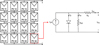Fig. 1 Formation of 4 × 4 solar arrays.

3 Mitigation techniques for the partial shading phenomenon

Numerous methods have been reported in the literature to mitigate power losses caused by PS. These methods are broadly categorized into two groups: (1) passive techniques and (2) active techniques, each encompassing several approaches, as illustrated in Figure 2.

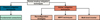Fig. 2 Detailed classification of PS mitigation techniques.

3.1 Passive mitigation techniques

In passive mitigation approaches, bypass diodes are the most widely employed components for alleviating the effects of PS. These diodes protect PV modules from excessive thermal stress and contribute to improved power extraction under shaded conditions. However, their presence introduces step-like behavior in the I–V characteristics and multiple peaks in the P–V curves of the PV array, as illustrated in Figures 3a and 3b, which correspond to two series-connected modules simulated under Partial Shading Conditions (PSC: PV1 at 1000 W/m² and PV2 at 700 W/m²) and Uniform Shading Conditions (USC: both the modules at 1000 W/m²), at 25°C. Among these peaks, only one corresponds to the GMPP, which yields the highest output power, while the remaining peaks represent local maxima [46].

In Figure 2, different types of conventional PV configurations PV array are presented. The series connection, commonly referred to as the simple series configuration or PV strings, is shown in Figure 4a [47]. Figure 4b illustrates the parallel configuration, where the PV modules are connected in parallel. As described in [48], combining series and parallel connections yields the series-parallel (SP) configuration, shown in Figure 4c. The total cross-tied (TCT) configuration is obtained by interconnecting the row junctions of the SP configuration through crossties, while the bridge-linked (BL) configuration arranges the modules in a bridge-like pattern, as depicted in Figures 4d and 4e [49]. Additionally, the hexagonal (HC) configuration arranges PV modules in a hexagonal layout, as shown in Figure 4f [50].

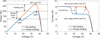Fig. 3 Solar losses under shading.

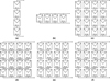Fig. 4 Classification of conventional PV array configurations: (a) S, (b) P, (c) SP, (d) TCT, (e) BL and (f) HC.

3.2 Active mitigation techniques

Active techniques have been demonstrated to be more effective than passive methods in mitigating the impact of PS in PV systems. These active approaches can be broadly classified into three categories: (1) Reconfiguration strategies, (2) MPPT techniques, and (3) Multi-level Inverter systems.

1) Reconfiguration strategies

PV module reconfiguration involves rearranging the modules according to irradiance levels to meet load requirements or operating conditions. This can be achieved either by altering module positions while keeping electrical connections unchanged or by modifying electrical connections while leaving module positions fixed [51–53]. This section discusses the two primary types of PV array reconfiguration: Electrical Array Reconfiguration (EAR) and Physical Array Reconfiguration (PAR).

• Electrical Array Reconfiguration: Under dynamic irradiance conditions, the Dynamic Photovoltaic Array Reconfiguration (DPVAR) continuously adapts the PV array configuration to maximize the power output. The proposed control architecture comprises a data acquisition (DAQ) system that collects the field measurements required by the PV mathematical model. The model estimates the unknown parameters and provides the necessary inputs to the reconfiguration process. Based on these inputs, the reconfiguration algorithm determines the optimal array configuration and generates the corresponding control signals for the switching matrix.

• Physical Array Reconfiguration: In static reconfiguration, the physical relocation of PV modules without altering electrical connections allows for the redistribution of shading effects and equalization of row current differences, thereby enhancing power output; this approach, eliminates the need for additional switching devices and simplifies the controller.

2) MPPT techniques

Maximum Power Point Tracking (MPPT) is employed to maximize the power output of a PV array under PSCs. The MPPT controller adjusts the duty cycle of the power converter to ensure extraction of the maximum possible power, effectively functioning as the control center of the tracking system [54,55].

3) Multilevel inverters

Multilevel inverters generate more than two voltage levels, which reduces output voltage harmonics and minimizes switching-related losses, enhancing overall efficiency of the system [56].

4 Advance reconfiguration strategies for mitigating partial shading effects in PV array

One of the key parameters in selecting a reconfiguration strategy is its economic viability, which necessitates a trade-off between efficiency and cost. Simple approaches typically require minimal computational resources and a limited number of sensors, making them cost-effective. In contrast, numerical and intelligent algorithms demand high-performance microcontrollers and extensive computational effort, thereby increasing implementation cost [44].

In this study, a static reconfiguration strategy is employed, incorporating several recently developed methods within this approach. Among conventional PV array interconnections, the TCT configuration is particularly effective, combining the benefits of both series and parallel connections, as shown in Figure 4a. Under PSCs, the TCT topology can extract higher power compared to other conventional configurations such as bridge-link, honeycomb, and triple-tied arrangements [7]. The row current (I_ROW) and total array voltage (V_ARRAY) for the TCT configuration are described by equation (2).

$${\text{I}}_{\text{ROW}}={\displaystyle \sum }_{\text{m}=1}^{\text{n}}{\text{I}}_{\text{row}\left(1\right)}\times {\text{ R}}_{1\text{m}}{\text{ and V}}_{\text{ARRAY}}={\displaystyle \sum }_{\text{m}=1}^{\text{n}}{\text{V}}_{\text{P}}.$$(2)

Based on certain mathematical principles, the aforementioned TCT configuration can be further reconfigured to overcome its existing limitations and enhance overall performance under PSC. Recent methods developed under this static reconfiguration framework include the following:

4.1 SHAPE-DO-KU puzzle (SPDK)

The SPDK puzzle is available in multiple grid sizes (e.g., 4 × 4, 5 × 5, and 6 × 6) and displays symmetrical properties. Although it is not directly related to the SDK puzzle, it can be viewed as a variant of the Latin Square (LS) [57] puzzle, with the constraint that each number must appear at least once in every row and column. In this study, the PV array is reconfigured using a 4 × 4 SPDK puzzle. The design methodology is presented in Figure 5, and the resulting solar module arrangement based on the SPDK topology is shown in Figure 13b.

Fig. 5 Flowchart of the SPDK methodology for designing 4x4 PV array [36].

4.2 Skyscraper reconfiguration (SS)

The SS puzzle is a logic-based number-placement game closely related to Sudoku. It is arranged on an m × n grid with clues positioned along the edges. Each module represents a skyscraper, and the goal is to assign heights from 1 to N to all modules such that no height is repeated in any row or column. Figure 6a shows a 4 × 4 SS puzzle, where the external clues indicate the number of skyscrapers visible from that viewpoint, with taller skyscrapers obscuring shorter ones behind them.

In the 4 × 4 grid, each of the 16 modules is influenced by its corresponding clue. The puzzle is solved as follows:

• Step 1: A clue of "4" means all four skyscrapers are visible, so the buildings are arranged in ascending order from 1 to 4, as shown in Figure 6b.

• Step 2: A clue of "1" indicates only the tallest skyscraper (height 4) is visible from that position, as demonstrated in Figure 6c.

• Step 3: A clue of "2" implies two skyscrapers are visible, so heights 3 and 4 are placed accordingly; placing height 1 would make all four skyscrapers visible, which is not allowed, as illustrated in Figure 6d.

The remaining modules are completed according to the provided clues, resulting in the final arrangement of solar modules in the SS topology, as shown in Figure 13c.

Fig. 6 Illustration of SS puzzle: (a) 4×4 grid with given clues, (b) row filled according to clue 4, (c) row filled according to clue 1, and (d) row filled according to clue 2 [37].

4.3 Ken-Ken reconfiguration (KK)

In 2021, the KK puzzle, a Sudoku-type logic game, was highlighted for enhancing reasoning and analytical skills. It uses an m × n grid divided into cages, each with a target value and arithmetic operation. For a 4 × 4 grid, numbers 1–4 are placed so that each appears only once per row and column, following the specified operations. Figure 7a shows the 4 × 4 puzzle used in this study. The puzzle is solved according to the following rules:

• Step 1: In the cage located in the second row, first column, a single-cell target of 2 is assigned. Therefore, this square is directly filled with the number 2.

• Step 2: In the cage in the fourth row, first column, the target value is 6 with an addition operation. Since number 2 is already present in that column, the remaining cells are filled with 1 and 3, completing the cage, as shown in Figure 7b.

• Step 3: In the cage in the first row, first column, the target value is 48 with a multiplication operation. The first column is filled with 4, and the remaining cells are filled with 1 and 3, as illustrated in Figure 7c.

• Step 4: The cages in the third and fourth columns are completed by applying their respective arithmetic operations (target value 10, addition), as shown in Figure 7d. The resulting arrangement for the KK-based PV reconfiguration is presented in Figure 13d.

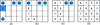Fig. 7 KK puzzle (a) initial layout, (b) arithmetic operations, (c) block filled using addition (2 + 6), (d) block filled using multiplication (48), (e) two blocks completed using arithmetic operation (10) [38].

4.4 Jigsaw reconfiguration (JS)

A JS puzzle-based method is proposed to rearrange PV modules in a 4 × 4 array to minimize mismatch losses under PSCs. The puzzle uses a 4 × 4 grid with four irregular regions, each containing numbers 1–4 without repetition in any row or column Figure 8a. The following steps outline the procedure for completing the puzzle:

• Step 1: Square 1 initially contains the numbers 1 and 3; thus, it can be completed by filling 2 and 4, as shown in Figure 8b. The first row of Block 2 is then filled with the number 1, as illustrated in Figure 8c.

• Step 2: The remaining blocks of Square 2 are filled with the numbers 2 and 3, while Square 3 in the first column is filled with the number 3, as depicted in Figure 8d.

• Step 3: Similarly, Square 4 is completed with the numbers 1 and 4, as shown in Figure 8e. The remaining squares are then filled accordingly, as presented in Figure 8f.

The final JS puzzle configuration, shown in Figure 13f, is used for subsequent analysis. In this arrangement, the first digit of each module label represents its position, while the second digit corresponds to its column number. For instance, in module 21, ‘2’ indicates the module position, and ‘1’ denotes the column. The PV array modules are then reorganized according to this JS puzzle layout, while maintaining the original electrical interconnections.

Fig. 8 (a – g) JS puzzle pattern [39].

4.5 Kendoku reconfiguration (KDT)

Proposed in 2023, the KDT method draws on the structural principles of both KenKen and Sudoku layouts to reduce power mismatch losses in PV arrays operating under non-uniform irradiance conditions. For an n × n array, integers 1 to n are assigned to module positions such that each integer appears exactly once in every row and column, while arithmetic constraints are applied within individual cages to govern number placement.

The reconfiguration is implemented according to the following steps:

• Step 1: Divide the n × n array into cages, each assigned a target value and an arithmetic operation (addition, subtraction, multiplication, or division).

• Step 2: Assign integers 1 to n to each cage so that every number appears exactly once per row and column, satisfying the Sudoku constraint.

• Step 3: Verify that all cage arithmetic constraints are satisfied simultaneously, ensuring a balanced electrical distribution across the array.

• Step 4: Map the physical PV modules to the reconfigured position indices. The resulting layout is presented in Figure 13f.

4.6 Novel Grecian reconfiguration (NGR)

Proposed in 2024, the NGR method is inspired by the symmetry and balance of ancient Greek architecture, adapted to PV array design to mitigate partial shading effects by uniformly redistributing the shadow pattern across the modules, thereby minimizing power losses.

For an m × n PV array, the reconfiguration is performed according to the following steps:

• Step 1: Arrange the first row of the array in sequential order.

• Step 2: Generate each subsequent row by applying a cyclic shift of module positions relative to the previous row, as illustrated in Figure 9.

• Step 3: Repeat the rotational process iteratively using the algorithm shown in Figure 10, updating module coordinates at each iteration while preserving matrix symmetry.

• Step 4: Verify that the final configuration produces a symmetrical and diversified layout, ensuring effective redistribution of modules under different shading patterns.

By applying this systematic permutation and rotation procedure, up to m! distinct configurations can be obtained for an m × n array. The final reconfigured layout is presented in Figure 13g.

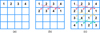Fig. 9 Partial placement of numbers on the Grecian board (b) rotation of numbers (c) completed novel Grecian board [41].

Fig. 10 Flowchart for novel reconfiguration (NGR) [41].

4.7 Novel Ramanujan reconfiguration (NRR)

Proposed in 2023, the NRR method arranges the positions of the PV modules in a symmetric matrix so that a constant sum of 10 is maintained across rows, columns, diagonals, corners, center, and specific sub-groups, as defined by equations (3)–(10). Specifically, equations (3) and (4) ensure row and column sums, equation (5) the diagonal sum, equation (6) the corner sum, equation (7) the central element sum, and equations (8)–(10) specific sub-group sums. The following conditions are required to be fulfilled:

$$\text{A}+\text{B}+\text{C}+\text{D},\text{ E}+\text{F}+\text{G}+\text{H},\text{ I}+\text{J}+\text{K}+\text{L},\text{ M}+\text{N}+\text{O}+\text{P}=10,$$(3)

$$\text{A}+\text{E}+\text{I}+\text{M},\text{ B}+\text{F}+\text{J}+\text{N},\text{ C}+\text{G}+\text{K}+\text{O},\text{ D}+\text{H}+\text{L}+\text{P}=10,$$(4)

$$\text{A}+\text{F}+\text{K}+\text{P},\text{ M}+\text{J}+\text{G}+\text{D}=10,$$(5)

$$\text{A}+\text{D}+\text{M}+\text{P}=10,$$(6)

$$\text{F}+\text{G}+\text{J}+\text{K}=10,$$(7)

$$\text{A}+\text{B}+\text{E}+\text{F},\text{ C}+\text{D}+\text{G}+\text{H},\text{ I}+\text{J}+\text{M}+\text{N},\text{ K}+\text{L}+\text{O}+\text{P}=10,$$(8)

$$\text{B}+\text{C}+\text{N}+\text{O},\text{ E}+\text{I}+\text{H}+\text{L}=10,$$(9)

$$\text{B}+\text{F}+\text{L}+\text{O},\text{ N}+\text{I}+\text{H}+\text{C}=10.$$(10)

The reconfiguration procedure, illustrated in the flowchart of Figure 11, follows three steps:

• Step 1: Iteratively search and swap pairs within matrix U until all constraint equations (3)–(10) are simultaneously satisfied.

• Step 2: Verify the isomorphic property through rotation, transposition, and row/column swapping, eliminating redundant reconfigurations.

• Step 3: Map the physical PV modules to the reconfigured position indices. The resulting layout is presented in Figure 13h.

Fig. 11 Step-wise configuration of the proposed SMR layout [43].

Fig. 12 Flowchart for novel reconfiguration (NRR) [42].

4.8 Novel super magic-square reconfiguration (SMR)

Proposed in 2025, the SMR method is based on constructing an n-order symmetric-caged matrix using the integer set (1 to n²), where a constant sum preserves symmetry across rows, columns, and diagonals. Unlike conventional TCT and earlier magic-square methods — which confine the module relocation to column-wise movements — SMR allows full-array module relocation, enabling effective shade dispersion over a wider area.

The reconfiguration is implemented according to the following steps:

• Step 1: Construct the n-order symmetric-caged matrix using integers 1 to n², ensuring the constant sum condition is satisfied across all rows, columns, and diagonals.

• Step 2: Apply systematic coordinate mapping with boundary-condition handling to iteratively relocate modules according to shading intensity, ensuring uniform irradiance mismatch distribution across the full array.

• Step 3: Identify optimal module positions through structured coordinate updates, minimizing shading concentration and enhancing power extraction. The overall reconfiguration process is illustrated in Figure 12.

• Step 4: Map the physical PV modules to the reconfigured positions. The resulting layout is presented in Figure 13i.

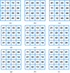Fig. 13 Wire connection for (a) TCT, (b) SPDK, (c) SS, (d) KK, (e) JS, (f) KDT, (g) NGR, (h) NRR, and (i) SMR.

5 Shading patterns and row current generation

Figure 14 depicts four realistic shading scenarios, viz., corner (S-1), half (S-2), tree (S-3), and chimney (S-4), that are considered in this study. The irradiance levels within the shaded regions vary between 100 and 1000 W/m². A total of 16 photovoltaic modules are arranged symmetrically and analyzed under multiple interconnection schemes, namely TCT, SPDK, SS, KK, JS, KDT, NGR, NRR, and SMR. During the sequential evaluation of these configurations(TCT→SPDK→ SS→KK→JS→KDT→NGR→NRR→ SMR), the shading distribution is applied uniformly across the array, as depicted for scenario S-1 in Figure 15.

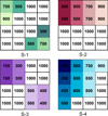Fig. 14 Four realistic shading scenarios.

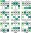Fig. 15 Shading distribution on the symmetrical 4 × 4 PV array under S-1.

5.1 Scenario-1 (S-1) Corner shading

For the corner-shading condition under consideration, the resulting row currents in the TCT configuration can be expressed using equations (11)–(13).

$$I_{R1}=I_{R4}=\left(\frac{700}{1000}\right)I_m+\left(\frac{500}{1000}\right)I_m+2\left(\frac{1000}{1000}\right)I_m=3.2I_m,$$(11)

$$I_{R2}=\left(\frac{900}{1000}\right)I_m+3\left(\frac{1000}{1000}\right)I_m=3.9I_m,$$(12)

$$I_{R3}=\left(\frac{300}{1000}\right)I_m+3\left(\frac{1000}{1000}\right)I_m=3.3I_m.$$(13)

The row currents for the SPDK interconnection scheme are determined using equations (14)–(17), which provide the corresponding analytical expressions.

$$I_{R1}=4\left(\frac{1000}{1000}\right)I_m=4I_m,$$(14)

$$I_{R2}=\left(\frac{1000}{1000}\right)I_m+2\left(\frac{500}{1000}\right)I_m+\left(\frac{1000}{1000}\right)I_m=3I_m,$$(15)

$$I_{R3}=\left(\frac{900}{1000}\right)I_m+2\left(\frac{1000}{1000}\right)I_m+\left(\frac{300}{1000}\right)I_m=3.2I_m,$$(16)

$$I_{R4}=\left(\frac{700}{1000}\right)I_m+2\left(\frac{1000}{1000}\right)I_m+\left(\frac{700}{1000}\right)I_m=3.4I_m.$$(17)

The row currents for the SS interconnection scheme are determined using equations (18)–(21), which provide the corresponding analytical expressions.

$$I_{R1}=4\left(\frac{1000}{1000}\right)I_m=4I_m,$$(18)

$$I_{R2}=\left(\frac{700}{1000}\right)I_m+3\left(\frac{1000}{1000}\right)I_m=3.7I_m,$$(19)

$$I_{R3}=3\left(\frac{1000}{1000}\right)I_m+\left(\frac{700}{1000}\right)I_m=3.7I_m,$$(20)

$$I_{R4}=\left(\frac{900}{1000}\right)I_m+2\left(\frac{500}{1000}\right)I_m+\left(\frac{300}{1000}\right)I_m=2.2I_m.$$(21)

The row currents for the KK interconnection scheme are determined using equations (22)–(25), which provide the corresponding analytical expressions.

$$I_{R1}=\left(\frac{1000}{1000}\right)I_m+\left(\frac{500}{1000}\right)I_m+2\left(\frac{1000}{1000}\right)I_m=3.5I_m,$$(22)

$$I_{R2}=\left(\frac{900}{1000}\right)I_m+\left(\frac{1000}{1000}\right)I_m+\left(\frac{500}{1000}\right)I_m+\left(\frac{1000}{1000}\right)I_m=3.4I_m,$$(23)

$$I_{R3}=\left(\frac{700}{1000}\right)I_m+2\left(\frac{1000}{1000}\right)I_m+\left(\frac{300}{1000}\right)I_m=3I_m,$$(24)

$$I_{R4}=3\left(\frac{1000}{1000}\right)I_m+\left(\frac{700}{1000}\right)I_m=3.7I_m.$$(25)

The row currents for the JS interconnection scheme are determined using equations (26)–(29), which provide the corresponding analytical expressions.

$$I_{R1}=\left(\frac{900}{1000}\right)I_m+2\left(\frac{1000}{1000}\right)I_m+\left(\frac{700}{1000}\right)I_m=3.6I_m,$$(26)

$$I_{R2}=\left(\frac{700}{1000}\right)I_m+3\left(\frac{1000}{1000}\right)I_m=3.7I_m,$$(27)

$$I_{R3}=\left(\frac{1000}{1000}\right)I_m+\left(\frac{500}{1000}\right)I_m+\left(\frac{1000}{1000}\right)I_m+\left(\frac{300}{1000}\right)I_m=2.8I_m,$$(28)

$$I_{R4}=2\left(\frac{1000}{1000}\right)I_m+\left(\frac{500}{1000}\right)I_m+\left(\frac{1000}{1000}\right)I_m=3.2I_m.$$(29)

The row currents for the KDT interconnection scheme are determined using equations (30)–(33), which provide the corresponding analytical expressions.

$$I_{R1}=\left(\frac{900}{1000}\right)I_m+\left(\frac{500}{1000}\right)I_m+\left(\frac{1000}{1000}\right)I_m+\left(\frac{700}{1000}\right)I_m=3.1I_m,$$(30)

$$I_{R2}=2\left(\frac{1000}{1000}\right)I_m+\left(\frac{500}{1000}\right)I_m+\left(\frac{1000}{1000}\right)I_m=3.5I_m,$$(31)

$$I_{R3}=\left(\frac{700}{1000}\right)I_m+2\left(\frac{1000}{1000}\right)I_m+\left(\frac{300}{1000}\right)I_m=3I_m,$$(32)

$$I_{R4}=4\left(\frac{1000}{1000}\right)I_m=4I_m.$$(33)

The row currents for the NGR interconnection scheme are determined using equations (34)–(37), which provide the corresponding analytical expressions.

$$I_{R1}=\left(\frac{700}{1000}\right)I_m+2\left(\frac{1000}{1000}\right)I_m+\left(\frac{700}{1000}\right)I_m=3.4I_m,$$(34)

$$I_{R2}=\left(\frac{900}{1000}\right)I_m+\left(\frac{1000}{1000}\right)I_m+\left(\frac{500}{1000}\right)I_m+\left(\frac{1000}{1000}\right)I_m=3.4I_m,$$(35)

$$I_{R3}=4\left(\frac{1000}{1000}\right)I_m=4I_m,$$(36)

$$I_{R4}=\left(\frac{1000}{1000}\right)I_m+\left(\frac{500}{1000}\right)I_m+\left(\frac{1000}{1000}\right)I_m+\left(\frac{300}{1000}\right)I_m=2.8I_m.$$(37)

The row currents for the NRR interconnection scheme are determined using equations (38)–(41), which provide the corresponding analytical expressions.

$$I_{R1}=\left(\frac{700}{1000}\right)I_m+2\left(\frac{1000}{1000}\right)I_m+\left(\frac{700}{1000}\right)I_m=3.4I_m,$$(38)

$$I_{R2}=4\left(\frac{1000}{1000}\right)I_m=4I_m,$$(39)

$$I_{R3}=\left(\frac{900}{1000}\right)I_m+2\left(\frac{500}{1000}\right)I_m+\left(\frac{300}{1000}\right)I_m=2.2I_m,$$(40)

$$I_{R4}=4\left(\frac{1000}{1000}\right)I_m=4I_m.$$(41)

The row currents for the SMR interconnection scheme are determined using equations (42)–(45), which provide the corresponding analytical expressions.

$$I_{R1}=\left(\frac{700}{1000}\right)I_m+\left(\frac{1000}{1000}\right)I_m+\left(\frac{500}{1000}\right)I_m+\left(\frac{1000}{1000}\right)I_m=3.2I_m,$$(42)

$$I_{R2}=\left(\frac{900}{1000}\right)I_m+3\left(\frac{1000}{1000}\right)I_m=3.9I_m,$$(43)

$$I_{R3}=3\left(\frac{1000}{1000}\right)I_m+\left(\frac{300}{1000}\right)I_m=3.3I_m,$$(44)

$$I_{R4}=\left(\frac{1000}{1000}\right)I_m+\left(\frac{500}{1000}\right)I_m+\left(\frac{1000}{1000}\right)I_m+\left(\frac{700}{1000}\right)I_m=3.2I_m.$$(45)

6 Evaluation of performance parameters

The performance indicators analyzed in this study are formally defined in Table 3, along with their corresponding mathematical expressions.

7 Results and discussions

The performance of static PV array reconfiguration techniques—Shape-Do-Ku (SDPK) [36], Skyscraper (SS) [37], Ken-Ken (KK) [38], Jigsaw (JS) [39], Kendoku (KDT) [40], Novel Grecian Reconfiguration (NGR) [41], Novel Ramanujan Reconfiguration (NRR) [42], Super Magic-Square Reconfiguration (SMR) [42], and conventional Total-Cross-Tied (TCT)—is evaluated under four realistic shading scenarios. The GMPP for each case is precisely identified using theoretical row-current computations. Performance is assessed via key indicators including Global Peak Power (GP), Shading Loss (SL), Fill Factor (FF), Efficiency Ratio (ER), and Power Gain (PG). Comparative analysis highlights each effectiveness of the method in mitigating mismatch losses and maximizing power extraction under non-uniform irradiance. All simulations are conducted in MATLAB R2023b/Simulink.

7.1 P-V and I-V curves at STC

The P–V and I–V characteristics of the PV module under standard test conditions and the irradiance distribution applied to the array are illustrated in Figure 16, as obtained from MATLAB simulations. The corresponding global maximum power point reaches 2148 W.

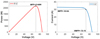Fig. 16 (a)-(b). P-Vand I-V curves (STC).

7.2 Corner shade (S-1)

When the S-1 shading pattern is applied to the 4 × 4 PV array, the resulting P–V and I–V characteristics shown in Figure 17, together with the quantitative results summarized in Table 4, indicate that the SMR, NRR, and TCT configurations achieve the highest power extraction. These are followed, in descending order, by KK, KDT, SPDK, JS, SS, and NGR. Although some configurations exhibit similar short-circuit currents, their maximum power outputs differ significantly due to the variations of the differences in the distribution of the current mismatch distribution and the resulting shape of the I–V and P–V characteristics. Therefore, the performance of a reconfiguration scheme under partial shading should be evaluated using the complete electrical characteristics of the array rather than relying solely on the short-circuit current or the minimum row current. The GP enhancement consequently improves the FF and reduces the SL, leading to a substantial enhancement in the performance of the overall system under the S-1 condition. Furthermore, a displaced GMPP may cause single-stage MPPT inverters to converge to a local maximum near the standard operating voltage, resulting in energy losses. The mathematical representation is given as follows:

$$\begin{array}{l}{\text{GP}}_{1776}^{\text{TCT}}={\text{ GP}}_{1776}^{\text{SMR}}={\text{GP}}_{1776}^{\text{NRR}}>{\text{GP}}_{1727}^{\text{KK}}>{\text{GP}}_{1722}^{\text{KDT}}={\text{GP}}_{1722}^{\text{SPDK}}>{\text{GP}}_{1644}^{\text{JS}}>{\text{GP}}_{1494}^{\text{SS}}>{\text{GP}}_{1490}^{\text{NGR}};\\ {\text{SL}}_{372}^{\text{TCT}}={\text{SL}}_{372}^{\text{SMR}}={\text{ SL}}_{372}^{\text{NRR}}<{\text{SL}}_{421}^{\text{KK}}<{\text{SL}}_{426}^{\text{KDT}}={\text{SL}}_{426}^{\text{SPDK}}<{\text{SL}}_{504}^{\text{JS}}<{\text{SL}}_{654}^{\text{SS}}<{\text{SL}}_{658}^{\text{NGR}};\\ {\text{FF}}_{63.90}^{\text{TCT}}={\text{FF}}_{63.90}^{\text{SMR}}={\text{FF}}_{63.90}^{\text{NRR}}>{\text{FF}}_{62.36}^{\text{JS}}>{\text{ FF}}_{62.14}^{\text{KK}}>{\text{FF}}_{60.40}^{\text{KDT}}={\text{FF}}_{60.40}^{\text{SPDK}}>{\text{FF}}_{52.41}^{\text{SS}}>{\text{FF}}_{52.27}^{\text{NGR}};\\ {\text{PR}}_{82.68}^{\text{TCT}}={\text{PR}}_{82.68}^{\text{SMR}}={\text{PR}}_{82.68}^{\text{NRR}}>{\text{PR}}_{80.40}^{\text{KK}}>{\text{PR}}_{80.16}^{\text{KDT}}={\text{PR}}_{80.16}^{\text{SPDK}}>{\text{PR}}_{76.53}^{\text{JS}}>{\text{PR}}_{69.55}^{\text{SS}}>{\text{PR}}_{69.36}^{\text{NGR}};\\ {\text{PG}}_{0.00}^{\text{SMR}}={\text{PG}}_{0.00}^{\text{NRR}}>{\text{PG}}_{-2.83}^{\text{KK}}>{\text{PG}}_{-3.13}^{\text{KDT}}={\text{PG}}_{-3.13}^{\text{SPDK}}>{\text{PG}}_{-8.02}^{\text{JS}}>{\text{PG}}_{-18.87}^{\text{SS}}>{\text{PG}}_{-19.19}^{\text{NGR}};\end{array}$$

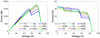Fig. 17 P-V and I-V curves for S-1.

7.3 Half shade (S-2)

The superior performance of NRR and SMR (GP = 1725 W) is attributed to their full-array module relocation capability, which distributes the shaded modules — concentrated in one half of the array — uniformly across all rows, minimizing current mismatch and bypass diode activation, as illustrated in Figure 18 and Table 4. TCT yields the lowest GP (1396 W) due to its fixed topology which concentrates shading losses on specific rows, producing a severely distorted P–V curve with multiple local maxima. The identical results of JS and KK (GP = 1693 W, FF = 69.88%) suggest equivalent shade dispersion for this specific shading pattern despite their different underlying algorithms. The mathematical formulation is given as follows:

$$\begin{array}{l}{\text{GP}}_{1725}^{\text{NRR}}={\text{ GP}}_{1725}^{\text{SMR}}>{\text{ GP}}_{1693}^{\text{JS}}={\text{GP}}_{1693}^{\text{KK}}>{\text{ GP}}_{1677}^{\text{SPDK}}>{\text{GP}}_{1619}^{\text{SS}}={\text{ GP}}_{1619}^{\text{NGR}}>{\text{GP}}_{1616}^{\text{KDT}}>{\text{GP}}_{1396}^{\text{TCT}};\\ {\text{SL}}_{423}^{\text{NRR}}={\text{ SL}}_{423}^{\text{SMR}}<{\text{ SL}}_{455}^{\text{JS}}={\text{SL}}_{455}^{\text{KK}}<{\text{SL}}_{471}^{\text{SPDK}}<{\text{SL}}_{529}^{\text{SS}}={\text{ SL}}_{529}^{\text{NGR}}<{\text{ SL}}_{533}^{\text{KDT}}<{\text{SL}}_{752}^{\text{TCT}};\\ {\text{FF}}_{75.56}^{\text{NRR}}={\text{ FF}}_{75.56}^{\text{SMR}}>{\text{FF}}_{69.88}^{\text{JS}}={\text{FF}}_{69.88}^{\text{KK}}>{\text{ FF}}_{69.17}^{\text{SPDK}}>{\text{FF}}_{63.10}^{\text{SS}}={\text{ FF}}_{63.10}^{\text{NGR}}>{\text{FF}}_{62.95}^{\text{KDT}}>{\text{FF}}_{48.94}^{\text{TCT}};\\ {\text{PR}}_{80.30}^{\text{NRR}}={\text{PR}}_{80.30}^{\text{SMR}}>{\text{PR}}_{78.81}^{\text{JS}}={\text{PR}}_{78.81}^{\text{KK}}>{\text{PR}}_{78.07}^{\text{SPDK}}>{\text{PR}}_{75.37}^{\text{SS}}={\text{PR}}_{75.37}^{\text{NGR}}>{\text{PR}}_{75.18}^{\text{KDT}}>{\text{PR}}_{64.99}^{\text{TCT}};\\ {\text{PG}}_{19.07}^{\text{NRR}}={\text{PG}}_{19.07}^{\text{SMR}}>{\text{PG}}_{17.54}^{\text{JS}}={\text{PG}}_{17.54}^{\text{KK}}>{\text{PG}}_{16.75}^{\text{SPDK}}>{\text{PG}}_{13.77}^{\text{SS}}={\text{PG}}_{13.77}^{\text{NGR}}>{\text{PG}}_{13.56}^{\text{KDT}};\end{array}$$

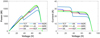Fig. 18 P-V and I-V curves for S-2.

7.4 Tree shade (S-3)

Under S-3, NRR and SMR again achieve the highest GP (1422 W), confirming their consistent superiority across diverse shading patterns due to their systematic irradiance redistribution across the full array, as shown in Figure 19 and Table 4. TCT no longer performs competitively under this more spatially complex shading pattern, as the tree shade affects multiple rows simultaneously, exposing the limitations of its fixed column-based topology. Notably, SS and NGR yield negative PG values (−23.9% and −26.9% respectively), indicating that these configurations perform worse than TCT under S-3, highlighting that not all reconfiguration methods are robust across different shading geometries. The mathematical representation is provided as follows:

$$\begin{array}{l}{\text{GP}}_{1422}^{\text{NRR}}={\text{ GP}}_{1422}^{\text{SMR}}>{\text{GP}}_{1404}^{\text{JS}}={\text{ GP}}_{1404}^{\text{KK}}>{\text{ GP}}_{1393}^{\text{SPDK}}>{\text{GP}}_{1353}^{\text{TCT}}>{\text{GP}}_{1092}^{\text{SS}}={\text{GP}}_{1092}^{\text{NGR}};>{\text{GP}}_{1066}^{\text{KDT}};\\ {\text{SL}}_{726}^{\text{NRR}}={\text{ SL}}_{726}^{\text{SMR}}<{\text{SL}}_{744}^{\text{JS}}={\text{SL}}_{744}^{\text{KK}}<{\text{SL}}_{755}^{\text{SPDK}}<{\text{SL}}_{795}^{\text{TCT}}<{\text{SL}}_{1056}^{\text{SS}}={\text{SL}}_{1056}^{\text{NGR}}<{\text{ SL}}_{1082}^{\text{KDT}};\\ {\text{FF}}_{73.85}^{\text{NRR}}={\text{ FF}}_{73.85}^{\text{SMR}}>{\text{FF}}_{70.40}^{\text{JS}}={\text{FF}}_{70.40}^{\text{KK}}>{\text{ FF}}_{69.78}^{\text{SPDK}}>{\text{FF}}_{65.44}^{\text{TCT}}>{\text{FF}}_{38.30}^{\text{SS}}={\text{ FF}}_{38.30}^{\text{NGR}};>{\text{FF}}_{37.39}^{\text{KDT}};\\ {\text{PR}}_{66.20}^{\text{NRR}}={\text{PR}}_{66.20}^{\text{SMR}}>{\text{PR}}_{65.36}^{\text{JS}}={\text{PR}}_{65.36}^{\text{KK}}>{\text{PR}}_{64.85}^{\text{SPDK}}>{\text{PR}}_{62.98}^{\text{TCT}}>{\text{PR}}_{50.83}^{\text{SS}}={\text{PR}}_{50.83}^{\text{NGR}};>{\text{PR}}_{49.62}^{\text{KDT}};\\ {\text{PG}}_{4.85}^{\text{NRR}}={\text{PG}}_{4.85}^{\text{SMR}}>{\text{PG}}_{3.63}^{\text{JS}}={\text{PG}}_{3.63}^{\text{KK}}>{\text{PG}}_{2.87}^{\text{SPDK}}>{\text{PG}}_{-23.9}^{\text{SS}}={\text{PG}}_{-23.9}^{\text{NGR}}>{\text{PG}}_{-26.9}^{\text{KDT}};\end{array}$$

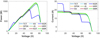Fig. 19 P-V and I-V curves for S-3.

7.5 Chimney shade (S-4)

Under S-4, SS, NGR, and NRR share the highest GP (1501 W), a result that departs from the consistent NRR/SMR dominance observed in S-1, S-2, and S-3, as presented in Figure 20 and Table 4. This demonstrates that the optimal reconfiguration strategy is shading-pattern dependent. The chimney shading pattern — which affects a narrow vertical strip of the array — particularly favors the configurations that disperse the PV modules along the row direction, explaining the strong performance of SS (2019) despite being the oldest method evaluated. SMR achieves a slightly lower GP (1475 W), suggesting that its magic-square based redistribution is marginally less effective for narrow vertical shading patterns compared to broader shading geometries. The mathematical formulation is expressed as follows:

$$\begin{array}{l}{\text{GP}}_{1501}^{\text{SS}}={\text{GP}}_{1501}^{\text{NGR}}={\text{GP}}_{1501}^{\text{NRR}}>{\text{GP}}_{1475}^{\text{SMR}}>{\text{GP}}_{1461}^{\text{JS}}>{\text{GP}}_{1460}^{\text{SPDK}}={\text{GP}}_{1460}^{\text{KK}}>{\text{GP}}_{1441}^{\text{KDT}}>{\text{GP}}_{1324}^{\text{TCT}};\\ {\text{SL}}_{647}^{\text{SS}}={\text{SL}}_{647}^{\text{NGR}}={\text{SL}}_{647}^{\text{NRR}}<{\text{SL}}_{673}^{\text{SMR}}<{\text{SL}}_{687}^{\text{JS}}<{\text{SL}}_{688}^{\text{SPDK}}={\text{SL}}_{688}^{\text{KK}}<{\text{ SL}}_{707}^{\text{KDT}}<{\text{SL}}_{824}^{\text{TCT}};\\ {\text{FF}}_{72.66}^{\text{SS}}={\text{FF}}_{72.66}^{\text{NGR}}={\text{FF}}_{72.66}^{\text{NRR}}>{\text{FF}}_{69.04}^{\text{SMR}}>{\text{FF}}_{70.66}^{\text{JS}}>{\text{FF}}_{69.47}^{\text{SPDK}}={\text{FF}}_{69.47}^{\text{KK}}>{\text{FF}}_{68.56}^{\text{KDT}}>{\text{FF}}_{53.08}^{\text{TCT}};\\ {\text{PR}}_{69.87}^{\text{SS}}={\text{PR}}_{69.87}^{\text{NGR}}={\text{PR}}_{69.87}^{\text{NRR}}>{\text{PR}}_{68.66}^{\text{SMR}}>{\text{PR}}_{68.01}^{\text{JS}}>{\text{PR}}_{67.97}^{\text{SPDK}}={\text{PR}}_{67.97}^{\text{KK}}>{\text{PR}}_{67.08}^{\text{KDT}}>{\text{PR}}_{61.63}^{\text{TCT}};\\ {\text{PG}}_{11.79}^{\text{SS}}={\text{PG}}_{11.79}^{\text{NGR}}={\text{PG}}_{11.79}^{\text{NRR}}>{\text{PG}}_{10.23}^{\text{SMR}}>{\text{PG}}_{9.37}^{\text{JS}}>{\text{PG}}_{9.31}^{\text{SPDK}}={\text{PG}}_{9.31}^{\text{KK}}>{\text{PG}}_{8.11}^{\text{KDT}};\end{array}$$

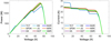Fig. 20 P-V and I-V curves for S-4.

7.6 Evaluation of performance parameters

a) Global peak power (GP)

Under uniform irradiance conditions, the PV array delivers a maximum power of 2148 W, which serves as the reference for comparative evaluation. The performance under partial shading scenarios (S-1 to S-4) reveals that the effectiveness of reconfiguration techniques strongly depends on the shading pattern and power dispersion among modules. The NRR, SMR, and TCT enhances GP by 3.04% (KDT, SPDK), 15.87% (SS), 2.75% (KK), 7.43% (JS), and 16.10% (NGR) during S-1; As S-2 the NRR, and SMR enhances GP by 19.07% (TCT), 2.78% (SPDK), 6.14% (SS, NGR), 1.85% (KK, JS), and 6.37% (KDT); 4.85% (TCT), 2.03% (SPDK), 23.20% (SS, NGR), 1.26% (KK, JS), and 25.03% (KDT) during S-3 respectively. Under S-4 the NRR, NGR, and SS enhances GP by 11.79% (TCT), 2.73% (SPDK, KK), 2.66% (JS), 3.99% (KDT), and 1.73% (SMR). Overall, these findings confirm that advanced reconfiguration strategies significantly improve GP extraction by minimizing mismatch losses and enhancing current distribution, as illustrated in Figure 21.

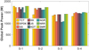Fig. 21 GP performance plot.

b) Shading Loss (SL)

Under uniform irradiance conditions, SL are absent, confirming ideal array operation. When partial shading is introduced, the mitigation capability of reconfiguration schemes becomes highly scenario-dependent. In scenario S-1, NRR, SMR, and TCT significantly reduce SL, achieving reductions of 14.51%, 14.51%, and 75.80%, respectively, outperforming SPDK, KDT, SS, KK, P-C, and NGR. This indicates that configurations with enhanced current redistribution are more effective under localized shading. As S-2 the NRR, and SMR mitigates SL by 77.77% (TCT), 11.34% (SPDK), 25.05% (SS, NGR), 7.56% (KK, JS), 26.00% (KDT), and 25.05% (NGR); 9.50% (TCT), 3.99% (SPDK), 45.45% (SS, NGR), 2.47% (KK, JS), and 49.03% (KDT) during S-3 respectively. Under S-4 the NRR, NGR, and SS mitigates SL by 27.35% (TCT), 6.33% (SPDK, KK), 6.18% (JS), 9.27% (KDT), and 4.01% (SMR), indicating that complex shading patterns restrict the effectiveness of static reconfiguration strategies. These trends are illustrated in Figure 22.

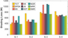Fig. 22 SL performance plot.

c) Fill Factor (FF)

The influence of array reconfiguration on the fill factor (FF) varies noticeably with the shading pattern. In scenario S-1, NRR, SMR, and TCT enhance FF by 5.47% for SPDK and KDT, 17.98% for SS, 2.75% for KK, 2.41% for JS, and 18.20% for NGR; As S-2 the NRR, and SMR increases FF by 35.23% (TCT), 8.45% (SPDK), 16.49% (SS, NGR), 7.51% (KK, JS), and 16.68% (KDT); 11.38% (TCT), 5.51% (SPDK), 48.13% (SS, NGR), 4.67% (KK, JS), and 49.37% (KDT) during S-3 respectively. Under S-4 the NRR, NGR, and SS increases FF by 26.94% (TCT), 4.39% (SPDK, KK), 2.75% (JS), 5.64% (KDT), and 4.98% (SMR). This confirms that severe and irregular shading reduces the effectiveness of static reconfiguration schemes. These results are summarized in Figure 23.

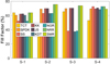Fig. 23 FF performance plot.

d) Performance Ratio (PR)

The impact of reconfiguration strategies on the PR demonstrates a strong dependence on the shading scenario. In S-1, NRR, SMR, and TCT enhance the performance of the overall system by 3.04%, 15.88%, 2.75%, 7.43%, 3.04%, and 16.11% when compared with SPDK, SS, KK, JS, KDT, and NGR, respectively. These improvements indicate more effective utilization of available irradiance under mild shading, primarily due to improved current balancing across rows. As S-2 the NRR, and SMR improved the PR by 19.06% (TCT), 2.77% (SPDK), 6.13% (SS, NGR), 1.85% (KK, JS), and 6.37% (KDT); 4.86% (TCT), 2.03% (SPDK), 23.21% (SS, NGR), 1.26% (KK, JS), and 25.04% (KDT) during S-3 respectively. Under S-4 the NRR, NGR, and SS improved the PR by 11.79% (TCT), 2.71% (SPDK, KK), 2.66% (JS), 3.99% (KDT), and 1.73% (SMR). This confirms that highly irregular shading constrains the effectiveness of static reconfiguration approaches. The comparative results are illustrated in Figure 24.

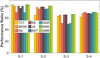Fig. 24 PR performance plot.

e) Power Gain (PG)

The NRR, and SMR has enhanced the power by 16.75% (SPDK), 13.77% (SS, NGR), 17.54% (KK, JS), and 28.89% (KDT) during S-2; 2.87% (SPDK), and 3.63% (KK, JS) during S-3; 9.31% (SPDK, KK), 11.79% (SS, NGR), 9.37% (JS), 31.21% (KDT), and 10.23% (SMR) during S-4, as illustrated in Figure 25.

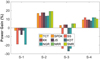Fig. 25 PG performance plot.

8 Conclusion

This study investigates mitigation strategies for PV arrays operating under PSCs through a comprehensive analysis of eight recently reported static reconfiguration schemes applied to a 4 × 4 PV array, namely SPDK, SS, KK, JS, KDT, NGR, NRR, and SMR. To ensure an objective evaluation, five key performance indicators—global peak power (GP), fill factor (FF), shading loss (SL), performance ratio (PR), and power gain (PG)—were systematically assessed. The comparative analysis demonstrates how these metrics vary in response to changing irradiance patterns and environmental conditions. The principal findings derived from this detailed investigation are summarized as follows:

• Under S-1, the NRR, SMR, and TCT configurations exhibit superior performance, achieving a GP improvement in the range of 2.75%–16.10% and enhancing the FF by up to 18.20%. Additionally, these configurations significantly reduce SL by 13.17%–76.88% when compared with the other reconfigured solar array models considered in this study.

• Under S-2 to S-3, the NRR, and SMR configurations maximize the GP between 1.26% and 25.03%, In addition, these configurations significantly reduce SL by 2.47%–77.77% and enhance the PR by 1.85%–19.06% compared with the other array layouts.

• Under S-4, more PG is attained by the proposed NRR, NGR, and SS (11.79%), followed by SPDK, KK (9.31%); JS (9.37%); KDT (8.11%); SMR (10.23%). These gains enhance the GP under non-uniform irradiance, with improvements ranging from 1.73% to 11.79%.

9 Future perspectives

By 2030, solar energy is expected to emerge as one of the most prominent and reliable sources for electrical power generation. Its large-scale deployment will contribute significantly to environmental sustainability by reducing greenhouse gas emissions and alleviating climate-related impacts. In this context, several future directions and research perspectives can be identified within the solar energy domain:

• Experimental validation on real PV installations is required to substantiate the simulation-based performance improvements.

• Daily and seasonal energy yield simulation using TMY (Typical Meteorological Year) irradiance profiles with sun-position-dependent shadow geometries.

• Experimental validation on a reduced-scale prototype, and extension to larger arrays (6 × 6 or 9 × 9).

• The development of hybrid reconfiguration strategies could improve robustness and adaptability under complex and highly variable partial shading scenarios.

• Scaling the approach through the interconnection of multiple reconfigured 4 × 4 PV arrays may facilitate deployment in commercial-scale systems and enhance overall energy yield.

• Detailed economic assessments, including wiring length, interconnection complexity, and installation costs, are necessary to evaluate practical feasibility and long-term viability.

Nomenclature

GMP: Global Maximum Power

AR: Array Reconfiguration

SL: Shading Loss (W)

PL: Power Loss (%)

FF: Fill Factor (%)

ER: Efficiency ratio (%)

PG: Power gain (%)

GP: Global peak power (W)

CL: Current loss (%)

TCT: Total cross-tied

L-S: L-shape

KDT: Kendoku

SPDK: SHAPE-DO-KU

ZZ: Zig-Zag

HC: Honeycomb

PAR: Physical Array Reconfiguration

SS: Skyscraper

LMP: Local Maximum Power

EAR: Electrical Array Reconfiguration

KK: Ken-Ken

MS: Magic Square

JS: Jigsaw

NGR: Novel Grecian Reconfiguration

SMR: Super Magic-square Reconfiguration

NRR: Novel Ramanujan Reconfiguration

LS: Latine Square

SP: Series-Parallel

OER: Odd-even

O-E-P: Odd–even-prime

PS: Partial shading

BL: Bridge-Link

STC: Standard Test Condition

DES: Dynamic Electrical Schemes

Acknowledgments

The authors are grateful to Mrs. Wilhelmina Logerais, a native English speaker, for her careful and thorough proofreading of the article.

Funding

This research has not received any external funding.

Conflicts of interest

The authors declare no conflict of interest.

Data availability statement

The data supporting the findings of this study will be made available upon reasonable request from the corresponding author after publication of the article.

Author contribution statement

Ilyas MIMOUN: Conceptualization, Methodology, Formal analysis, Validation, Data curation, Writing – original draft, Visualization; Youcef MIHOUB: Supervision, Writing – review & editing; Pierre-Olivier LOGERAIS: Methodology, Data curation, Writing – review & editing; Khairullah Mohammed KARAM: Methodology, Formal analysis, Writing – review & editing; Mahamadou ABDOU TANKARI: Supervision; Aicha ASRI: Supervision; Said HASSAINE: Supervision.

References

All Tables

All Figures

	Fig. 1 Formation of 4 × 4 solar arrays.
In the text

	Fig. 2 Detailed classification of PS mitigation techniques.
In the text

	Fig. 3 Solar losses under shading.
In the text

	Fig. 4 Classification of conventional PV array configurations: (a) S, (b) P, (c) SP, (d) TCT, (e) BL and (f) HC.
In the text

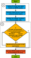	Fig. 5 Flowchart of the SPDK methodology for designing 4x4 PV array [36].
In the text

	Fig. 6 Illustration of SS puzzle: (a) 4×4 grid with given clues, (b) row filled according to clue 4, (c) row filled according to clue 1, and (d) row filled according to clue 2 [37].
In the text

	Fig. 7 KK puzzle (a) initial layout, (b) arithmetic operations, (c) block filled using addition (2 + 6), (d) block filled using multiplication (48), (e) two blocks completed using arithmetic operation (10) [38].
In the text

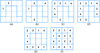	Fig. 8 (a – g) JS puzzle pattern [39].
In the text

	Fig. 9 Partial placement of numbers on the Grecian board (b) rotation of numbers (c) completed novel Grecian board [41].
In the text

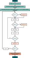	Fig. 10 Flowchart for novel reconfiguration (NGR) [41].
In the text

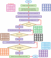	Fig. 11 Step-wise configuration of the proposed SMR layout [43].
In the text

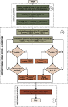	Fig. 12 Flowchart for novel reconfiguration (NRR) [42].
In the text

	Fig. 13 Wire connection for (a) TCT, (b) SPDK, (c) SS, (d) KK, (e) JS, (f) KDT, (g) NGR, (h) NRR, and (i) SMR.
In the text

	Fig. 14 Four realistic shading scenarios.
In the text

	Fig. 15 Shading distribution on the symmetrical 4 × 4 PV array under S-1.
In the text

	Fig. 16 (a)-(b). P-Vand I-V curves (STC).
In the text

	Fig. 17 P-V and I-V curves for S-1.
In the text

	Fig. 18 P-V and I-V curves for S-2.
In the text

	Fig. 19 P-V and I-V curves for S-3.
In the text

	Fig. 20 P-V and I-V curves for S-4.
In the text

	Fig. 21 GP performance plot.
In the text

	Fig. 22 SL performance plot.
In the text

	Fig. 23 FF performance plot.
In the text

	Fig. 24 PR performance plot.
In the text

	Fig. 25 PG performance plot.
In the text

References

- A. Gupta, Y.K. Chauhan, Detailed performance analysis of realistic solar photovoltaic systems at extensive climatic conditions, Energy 116, 716 (2016) [Google Scholar]
- P.K. Pathak, A.K. Yadav, P.A. Alvi, Advanced solar MPPT techniques under uniform and non-uniform irradiance: a comprehensive review, J. Sol. Energy Eng. 142, 040801 (2020). https://doi.org/10.1115/1.4046090 [Google Scholar]
- M. Seyed Mahmoudian, T.K. Soon, B. Horan, A. Ghandhari, S. Mekhilef, A. Stojcevski, New ARMO-based MPPT technique to minimize tracking time and fluctuation at the output of PV systems under rapidly changing shading conditions, in IEEE Transactions on Industrial Informatics (2019) [Google Scholar]
- M.M.A. Awan, A.B. Asghar, M.Y. Javed, Z. Conka, Ordering technique for the maximum power point tracking of an islanded solar photovoltaic system, Sustainability 15, 3332 (2023) [Google Scholar]
- D. Yousri, T.S. Babu, D. Allam, V.K. Ramach, A.M.B. Etiba, A novel chaotic flower pollination algorithm for global maximum power point tracking for photovoltaic systems under partial shading conditions, IEEE Access 7, 121432 (2019) [Google Scholar]
- D. Yousri, T.S. Babu, S. Mirjalili, N. Rajasekar, M.A. Elaziz, A novel objective function with artificial ecosystem-based optimization to reduce mismatch power loss in large-scale photovoltaic arrays, Energy Convers. Manage. 225, 113385 (2020) [Google Scholar]
- R.K. Pachauri, I. Kansal, T.S. Babu, H.H. Alhelou, Power losses reduction of solar PV systems under partial shading conditions using re-allocation of PV module-fixed electrical connections, IEEE Access 9, 94789 (2021), https://doi.org/10.1109/ACCESS.2021.3093954 [Google Scholar]
- A.M. Ajmal, T.S. Babu, V.K. Ramachandaramurthy, D. Yousri, J.B. Ekanayake, Approaches for mitigating the effects of partial shading on photovoltaic arrays using static and dynamic reconfiguration, Sustain. Energy Technol. Assess. 40, 100738 (2020) [Google Scholar]
- D. Prince Winston, K. Ganesan, P.K.B.D. Samithas, C.B. Baladhanautham, Experimental investigation on output power enhancement of partial shaded solar photovoltaic system, Energy Sources A Recovery Util. Environ. Eff. 117, 9793 (2020) [Google Scholar]
- T.S. Babu, D. Yousri, K. Balasubramanian, Photovoltaic array reconfiguration system for maximizing the harvested power using population-based algorithms, IEEE Access 8, 109608109624 (2020) [Google Scholar]
- G. Velasco-Quesada, F. Guinjoan-Gispert, R. Pique-Lopez, M. Roman-Lumbreras, A. Conesa-Roca, Electrical PV array reconfiguration strategy for energy extraction improvement in grid connected PV systems, IEEE Trans. Ind. Electron. 56, 43194331 (2009) [Google Scholar]
- E.R. Sanseverino, T.N. Ngoc, M. Cardinale, V. Li Vigni, D. Musso, P. Romano, F. Viola, Dynamic programming and munkres algorithm for optimal photovoltaic arrays reconfiguration, Sol. Energy 122, 347358 (2015) [Google Scholar]
- M. Karakose, K. Murat, E. Akin, K.S. Parlak, A new efficient reconfiguration approach based on genetic algorithm in PV systems, in Proc. IEEE 23rd Int. Symp. Ind. Electron. (ISIE) (2014), p. 2328 [Google Scholar]
- V.S. Bhadoria, R.K. Pachauri, S. Tiwari, S.P. Jaiswal, H.H. Alhelou, Investigation of different BPD placement topologies for shaded modules in a series-parallel configured PV array, IEEE Access 8, 216911216921 (2020) [Google Scholar]
- R. Singh, V.K. Yadav, M. Singh, A comprehensive shade resilient approach for enhanced PV array performance under irradiance mismatch conditions, IEEE J. Photovoltaics 14, 549 (2024), https://doi.org/10.1109/jphotov.2024.3374069 [Google Scholar]
- V. Jain, V. Kumar, S. Garg, V.K. Yadav, Cyclic heap permutation based reconfiguration of solar PV array for optimal shade dispersion, in 2024 11th International Conference on Signal Processing and Integrated Networks (SPIN) (IEEE, Noida, India, 2024), p. 245, https://doi.org/10.1109/SPIN60856.2024.10511429 [Google Scholar]
- F. Ameen, A. Troh´ak, A. Siddiq, R. Benotsmane, Enhancing photovoltaic array performance under partial shading through dynamic reconfiguration and layer equalization algorithm, in 2024 25th International Carpathian Control Conference (ICCC) (Krynica Zdr´ oj, Poland, IEEE, 2024), pp. 1–6, https://doi.org/10.1109/ICCC62069.2024.10569654 [Google Scholar]
- R.K. Pachauri, J.G. Singh, A novel approach for solar PV modules reconfiguration to achieve GMPP from partially-shaded PV array system: an experimental analysis, in 2022 22nd National Power Systems Conference (NPSC) (IEEE, New Delhi, India, 2022), p. 266, https://doi.org/10.1109/NPSC57038.2022.10069630 [Google Scholar]
- T.S. Babu, J.P. Ram, T. Dragicevic, M. Miyatake, F. Blaabjerg, N. Rajasekar, Particle swarm optimization based solar PV array reconfiguration of the maximum power extraction under partial shading conditions, IEEE Trans. Sustain. Energy 9, 74 (2018), https://doi.org/10.1109/TSTE.2017.2714905 [Google Scholar]
- S.N. Deshkar, S.B. Dhale, J.S. Mukherjee, T.S. Babu, N. Rajasekar, Solar PV array reconfiguration under partial shading conditions for maximum power extraction using genetic algorithm, Renew. Sustain. Energy Rev. 43, 102 (2015), https://doi.org/10.1016/j.rser.2014.10.098 [Google Scholar]
- B. Yang et al., PV arrays reconfiguration for partial shading mitigation: recent advances, challenges and perspectives, Energy Convers. Manag. 247, 114738 (2021), https://doi.org/10.1016/j.enconman.2021.114738 [Google Scholar]
- G. Sai Krishna, T. Moger, A novel adaptive dynamic photovoltaic reconfiguration system to mitigate mismatch effects, Renew. Sustain. Energy Rev. 141, 110754 (2021), https://doi.org/10.1016/j.rser.2021.110754 [Google Scholar]
- D. Mathew et al., Parameter estimation of organic photovoltaic cells – a three-diode approach using wind-driven optimization algorithm, IEEE J. Photovoltaics 12, 327 (2022), https://doi.org/10.1109/JPHOTOV.2021.3129874 [Google Scholar]
- K.T. Swetha, B. Venugopal Reddy, An effective dual-objective optimization to enhance power generation in a two-stage grid-tied PV system under partial shading conditions, Energy 305, 132259 (2024), https://doi.org/10.1016/j.energy.2024.132259 [Google Scholar]
- A.S. Yadav, V. Mukherjee, Comprehensive investigation of various bypass diode associations for killer-SuDoKu PV array under several shading conditions, Energy 239, 122014 (2022), https://doi.org/10.1016/j.energy.2021.122014 [Google Scholar]
- D.S. Pillai, J.P. Ram, J.L. Garcia, Y.-J. Kim, J.P.S. Catal˜ao, Experimental studies on a new array design and maximum power tracking strategy for enhanced performance of soiled photovoltaic systems, IEEE Trans. Power Electron. 39, 1596 (2024), https://doi.org/10.1109/TPEL.2023.3321601 [Google Scholar]
- P.K. Kesavan, A. Karthikeyan, M. Kumar, S. Mandal, A simple primary key algorithm based shade dispersion method for maximizing PV power generation under partial shading conditions, Chin. J. Electr. Eng. 10, 93 (2024), https://doi.org/10.23919/CJEE.2024.000067 [Google Scholar]
- R. Candela, E.R. Sanseverino, P. Romano, M. Cardinale, D. Musso, A dynamic electrical scheme for the optimal reconfiguration of PV modules under non-homogeneous solar irradiation, Appl. Mech. Mater. 197, 768 (2012). https://doi.org/10.4028/www.scientific.net/AMM.197.768 [Google Scholar]
- B.I. Rani, G.S. Ilango, C. Nagamani, Enhanced power generation from PV array under partial shading conditions by shade dispersion using sudoku configuration, IEEE Trans. Sustain. Energy 4, 594601 (2013) [Google Scholar]
- M. Horouany, R. Ghandehari, Optimization of the sudoku based reconfiguration technique for PV arrays power enhancement under mutual shading conditions, Sol. Energy 159, 10371046 (2018) [Google Scholar]
- H.S. Sahu, S.K. Nayak, S. Mishra, Maximizing the power generation of a partially shaded PV array, IEEE J. Emerg. Sel. Top. Power Electron. 4, 626637 (2016) [Google Scholar]
- A.S. Yadav, R.K. Pachauri, Y.K. Chauhan, S. Choudhury, R. Singh, Performance enhancement of partially shaded PV array using novel shade dispersion effect on magic-square puzzle configuration, Sol. Energy 144, 780797 (2017) [Google Scholar]
- S. Vijayalekshmy, G.R. Bindu, S.R. Iyer, A novel Zig-Zag scheme for power enhancement of partially shaded solar arrays, Sol. Energy 135, 92102 (2016) [Google Scholar]
- N. Belhaouas, M.-S.-A. Cheikh, P. Agathoklis, M.-R. Oularbi, B. Amrouche, K. Sedraoui, N. Djilali, PV array power output maximization under partial shading using new shifted PV array arrangements, Appl. Energy 187, 326337 (2017) [Google Scholar]
- B. Dhanalakshmi, N. Rajasekar, Dominance square-based array reconfiguration scheme for power loss reduction in solar PhotoVoltaic (PV) systems, Energy Convers. Manage. 156, 84102 (2018) [Google Scholar]
- R.K. Pachauri, I. Kansal, T.S. Babu, H.H. Alhelou, Power losses reduction of solar PV systems under partial shading conditions using re-allocation of PV module-fixed electrical connections, IEEE Access 9, 94789 (2021), https://doi.org/10.1109/access.2021.3093954 [Google Scholar]
- M. Palpandian, D.P. Winston, B.P. Kumar, C.S. Kumar, T.S. Babu, H.H. Alhelou, A new ken-ken puzzle pattern based reconfiguration technique for maximum power extraction in partial shaded solar PV array, IEEE Access 9, 65824 (2021), https://doi.org/10.1109/access.2021.3076608 [Google Scholar]
- G.S. Krishna, T. Moger, Enhancement of maximum power output through reconfiguration techniques under non-uniform irradiance conditions, Energy 187, 115917 (2019), https://doi.org/10.1016/j.energy.2019.115917 [Google Scholar]
- P.M. et al., A jigsaw puzzle based reconfiguration technique for enhancing maximum power in partial shaded hybrid photovoltaic array (May 18, 2021). https://doi.org/10.21203/rs.3.rs-513975/v1 [Google Scholar]
- D. Bonkoungou, T. Guingane, E. Korsaga, S. Tassembedo, Z. Koalaga, A. Darga, F. Zougmore, A novel topology to improve PV module efficiency under partial shading conditions, Int. J. Photoenergy 2022, 4401187 (2022) [Google Scholar]
- V.L. Mishra, Y.K. Chauhan, K.S. Verma, Attenuation of shading loss using a novel solar array reconfigured topology under partial shading conditions, Sol. Energy 274, 112552 (2024), https://doi.org/10.1016/j.solener.2024.112552 [Google Scholar]
- V.L. Mishra, Y.K. Chauhan, K.S. Verma, A novel reconfiguration of the solar array to enhance peak power and efficiency under partial shading conditions: experimental validation, Clean Energy 7, 824 (2023) [Google Scholar]
- V.L. Mishra, Y.K. Chauhan, K.S. Verma, R.S. Bajpai, Optimized reconfiguration scheme for a photovoltaic system to boost global peak power under realistic shading conditions: experimental validation, Exp. Syst. Appl. 296, 129263 (2026), https://doi.org/10.1016/j.eswa.2025.129263 [Google Scholar]
- M.A. Danandeh, Comparative and comprehensive review of maximum power point tracking methods for PV cells, Renew. Sustain. Energy Rev. 82, 2743 (2018) [Google Scholar]
- V.L. Mishra, Y.K. Chauhan, K.S. Verma, Various modeling approaches of photovoltaic module: a comparative analysis, Majlesi J. Electr. Eng. 17, 117 (2023) [Google Scholar]
- C. Larbes, S.M. Aït Cheikh, T. Obeidi, A. Zerguerras, Genetic algorithms optimized fuzzy logic control for the maximum power point tracking in photovoltaic system, Renew. Energy 34, 2093 (2009), https://doi.org/10.1016/j.renene.2009.01.006 [CrossRef] [Google Scholar]
- H.S. Rauschenbach, Electrical output of shadowed solar arrays, IEEE Trans. Electron Devices 18, 483 (1971), https://doi.org/10.1109/T-ED.1971.17231 [Google Scholar]
- J.W. Bishop, Computer simulation of the effects of electrical mismatches in photovoltaic cell interconnection circuits, Sol. Cells 25, 73 (1988), https://doi.org/10.1016/0379-6787(88)90059-2 [Google Scholar]
- N.K. Gautam, N.D. Kaushika, An efficient algorithm to simulate the electrical performance of solar photovoltaic arrays, Energy 27, 347 (2002), https://doi.org/10.1016/S0360-5442(01)00089-5 [Google Scholar]
- Y.-J. Wang, P.-C. Hsu, An investigation on partial shading of PV modules with different connection configurations of PV cells, Energy 36, 3069 (2011), https://doi.org/10.1016/j.energy.2011.02.052 [Google Scholar]
- G.H.K. Varma, V.R. Barry, R.K. Jain, D. Kumar, An MMTES algorithm for dynamic photovoltaic array reconfiguration to enhance power output under partial shading conditions, IET Renew. Power Gen. 15, 809 (2021), https://doi.org/10.1049/rpg2.12070 [Google Scholar]
- Y. Jiang, J. Xu, X. Leng, N. Eghbalian, RETRACTED: a novel hybrid maximum power point tracking method based on improving the effectiveness of different configuration partial shadow, Sustain. Energy Technol. Assess. 50, 101835 (2022), https://doi.org/10.1016/j.seta.2021.101835 [Google Scholar]
- B. Yang et al., Socio-inspired democratic political algorithm for optimal PV array reconfiguration to mitigate partial shading, Sustain. Energy Technol. Assess. 48, 101627 (2021), https://doi.org/10.1016/j.seta.2021.101627 [Google Scholar]
- Hybrid, optimization, intelligent and classical PV MPPT techniques: review (CSEE JPES, 2020), https://doi.org/10.17775/CSEEJPES.2019.02720 [Google Scholar]
- A. Al Mansur, Md. R. Amin, Performance investigation of different PV array configurations at partial shading condition for maximum power output, in 2019 International Conference on Sustainable Technologies for Industry 4.0 (STI) (IEEE, Dhaka, Bangladesh, Dec. 2019), pp. 1–5. https://doi.org/10.1109/STI47673.2019.9067998 [Google Scholar]
- M.D. Siddique, S. Mekhilef, N.M. Shah, A. Sarwar, A. Iqbal, M.A. Memon, A new multilevel inverter topology with reduce switch count, IEEE Access 7, 58584 (2019), https://doi.org/10.1109/ACCESS.2019.2914430 [Google Scholar]
- R. Pachauri, A.S. Yadav, Y.K. Chauhan, A. Sharma, V. Kumar, Performance enhancement in photovoltaic array configurations under partial shading using shade dispersion techniques, Int. Trans. Electr. Energy Syst. 28, e2556 (2018) [Google Scholar]
- V.L. Mishra, Y.K. Chauhan, K.S. Verma, A critical review on advanced reconfigured models and metaheuristics-based MPPT to address complex shadings of solar array, Energy Conver. Manage. 269, 116099 (2022) [Google Scholar]
- V.L. Mishra, Y.K. Chauhan, K.S. Verma, A new physics-based solar reconfigured model to enhance efficiency under partial shading conditions: experimental feasibility, Int. J. Green Energy 21, 589 (2023) [Google Scholar]
- G. Sagar, D. Pathak, P. Gaur, V. Jain, A Su Do Ku puzzle-based shade dispersion for maximum power enhancement of partially shaded hybrid bridge-link-total-cross-tied PV array, Sol. Energy 204, 161 (2020) [Google Scholar]
Cite this article as: Ilyas Mimoun, Youcef Mihoub, Pierre-Olivier Logerais, Khairullah Mohammed Karam, Mahamadou Abdou Tankari, Aicha Asri, Said Hassaine, Performance assessment of advanced static reconfiguration strategies to address realistic shading of solar arrays, EPJ Photovoltaics 17, 24 (2026), https://doi.org/10.1051/epjpv/2026016