| Issue |
EPJ Photovolt.
Volume 14, 2023
Special Issue on ‘Recent Advances in Spectroscopy and Microscopy of Thin-films Materials, Interfaces, and Solar Cells 2021', edited by A. Vossier, M. Gueunier-Farret, J.-P. Kleider and D. Mencaraglia
|
|
|---|---|---|
| Article Number | 40 | |
| Number of page(s) | 13 | |
| Section | Semiconductor Thin Films | |
| DOI | https://doi.org/10.1051/epjpv/2023031 | |
| Published online | 22 December 2023 | |
https://doi.org/10.1051/epjpv/2023031
Original Article
Investigations on photovoltaic material absorptivity using hyperspectral photoluminescence excitation imaging
1
EDF R&D, 91120 Palaiseau, France
2
Institut Photovoltaïque d'Ile de France (IPVF), 91120 Palaiseau, France
3
UMR IPVF 9006, CNRS, Ecole Polytechnique Institut Polytechnique de Paris, PSL Chimie ParisTech, IPVF SAS, 91120 Palaiseau, France
4
Lumière, Matière et Interfaces (LuMIn) Laboratory, Université Paris-Saclay, ENS Paris-Saclay, CNRS, CentraleSupelec, 91190 Gif-sur-Yvette, France
* e-mail: This email address is being protected from spambots. You need JavaScript enabled to view it.
Received:
29
June
2022
Received in final form:
29
September
2023
Accepted:
16
November
2023
Published online: 22 December 2023
Abstract
Photoluminescence imaging has become a standard method to characterize solar cells. However, performing some quantitative analysis of this technique requires the assumption of uniform local absorptivity, which cannot be directly measured using traditional methods. This study presents a novel approach to measure the local relative absorptivity over a broad spectral range for a perovskite absorber deposited on a charge extraction layer and an electrode. By analyzing the photoluminescence intensity as a function of the incident photon energy, we were able to determine the relative absorptivity of the incident light above the bandgap energy. Additionally, luminescence spectra allow us to accurately assess the absorptivity near the bandgap energy from the reciprocity between absorption and emission. Reflectivity measurements were also performed to further understand the possible limitations of our experiment and to discuss our results. Finally, this method was able to distinguish between variations in the photoluminescence response caused by slight differences in the local film thickness and changes in the local carrier lifetime.
Key words: Hyperspectral imaging / photoluminescence excitation spectroscopy / absorptivity / reflectance
© M. Legrand et al., Published by EDP Sciences, 2023
 This is an Open Access article distributed under the terms of the Creative Commons Attribution License (https://creativecommons.org/licenses/by/4.0), which permits unrestricted use, distribution, and reproduction in any medium, provided the original work is properly cited.
1 Introduction
The maximum energy conversion efficiency of a solar cell is determined by the absorptivity of its absorber, which quantifies the generation of electron-hole pairs in the device. It is thus a key parameter to assess the optical optimization of the different layers of the solar cell. Various optical models [1,2] help estimate the absorption coefficient from this quantity. This material property determines the depth-dependent electronic generation and is necessary to thoroughly understand the cell optoelectronic characteristics. Through its dependence on the electronic density of states, the absorption coefficient reflects not only the chemical composition of the material but also offers valuable information on its sub-bandgap properties such as Urbach energy, which influence the material optoelectronic performance by increasing the probability of non-radiative recombination. Especially relevant for the case of thin film absorbers, the sub-bandgap absorption is known to reflect at least the structural and thermal disorder at the lattice scale and is involved in performance losses of the material. Sub-bandgap absorptivity might also be influenced by shallow trap-state density depending on its energy distribution [3].
The absorption properties also have an impact on photoluminescence (PL) imaging and their variation must be assessed to achieve an accurate interpretation of PL images. Inhomogeneous PL images raise questions about the relationship between the brightness of certain areas and the device properties. Is the brightness due to higher absorption, resulting in a higher concentration of generated carriers, or is it due to a superior coefficient for radiative emission? Alternatively, could it be a result of lower non-radiative recombination? In such a case, it is necessary to discuss the traditional assumption of perfect incident light absorption. A precise estimation of the absorption coefficient is essential for determining material properties such as diffusion coefficient, carrier lifetime, or surface recombination velocity as long as all these properties significantly influence the carrier density profile in time-resolved or steady-state experiments.
Accurately measuring the absorption properties presents numerous challenges. In particular, the exponential increase of the absorption coefficient in the near vicinity of the bandgap energy requires the precise measurement of ultralow coefficients. In addition to this, classical techniques, such as reflectance and transmittance measurements, are sensitive to parasitic absorption by all layers of the stack. As an alternative, ellipsometry allows for the determination of the complex refraction index but needs oscillator models and partially void layers to reflect the material surface imperfection. Despite of great interest, these methods provide data averaged on large surfaces. Getting access to spatially resolved absorption properties, which is important for very inhomogeneous materials such as perovskite thin films, requires new methods. Furthermore, absorption properties vary with charge carriers' densities [4] or temperature, and thus with the experimental conditions. Directly accessing the absorptivity through luminescence for luminescence images interpretation guarantees the same environment and offers many advantages in addressing these challenges.
The PL emission, due to the exponential blackbody prefactor leveling the absorption drop around bandgap energy, has been used successfully to determine ultralow absorption coefficient values in the vicinity of the bandgap energy [5–7]. Otherwise, photoluminescence excitation (PLE) spectroscopy offers insight into the sample absorptivity by analyzing the intensity emitted with varied incident photon energies [8,9], within a complementary spectral range. In the case of PLE experiments, the photoluminescence emission allows for probing the absorptivity, and therefore absorption coefficient, in specific emitting layers. This is of interest for quantum structures whose absorption properties of the different layers can be explored without any structural modification, as pointed out by Jimenez [10]. It may be useful in case of low absorption for which transmission measurements cannot distinguish the materials. However, PL may still be affected by parasitic absorption, such as the one from the layers above the emitter [11]. Finally, PL imaging techniques are available, providing a means to assess spatial inhomogeneities and determine the local absorptivity of photovoltaic materials [12,13].
In the present work, PL hyperspectral acquisitions are performed with different excitation energies to obtain the local emission spectra. This data allows us to assess the shape of the local absorptivity close to the bandgap energy based on absorption-emission reciprocity. Complementarily, the variation in intensity with the excitation energy provides information on the absorptivity of the illumination, at energies higher than the bandgap. Firstly, the theoretical framework of this study is set, and the link between the PLE and absorptivity is derived for limiting cases. In the second part, the experimental methodology is detailed and our physical model is further supported by drift-diffusion simulations. The results of PL fit and PLE are compared, and their ability to assess absorptivity and lifetime images is discussed.
2 Theoretical background
During PL experiments, the sample undergoes excitation by a monochromatic light flux, indicated as Φexc. The PLE spectra are defined by the proportion of externally emitted photon flux, denoted as Φem, to the incident one, for varying excitation energy Eexc, reading:
 (1)
(1)
It is worth noting that this quantity is influenced by the absorptivity of the top layers in the incident light bandwidth, in the same way as the absorptivity of the emitter layer. Additionally, it is affected in the PL emission spectral range, resulting in an extra transmission coefficient.
As shown in Figure 1, PLE has to be distinguished from the spectrally resolved PL emission. Indeed, the PLE absolute value can be obtained by integrating the entire spectral emission. Under the assumption of a PL spectrum spectrally stable with the excitation energy sometimes implied in the literature [10], PLE relative value can be measured by optically filtering a specified spectral range of PL emission and monitoring its intensity.
The higher the absorptivity at the excitation energy in the absorber layer A (Eexc) = Aexc, the more PL is emitted. As such, they are very similar to External Quantum Efficiency (EQE) measurements that also assess the response of the device for different illumination energies, yet through the generated current. If the latter depends on the collection of the carriers, the former relies on the ability of the device to convert the generated carriers into photons through photoluminescence. Indeed, when operating in a low injection regime where photoluminescence is directly proportional to the density of minority carriers, and assuming that all spontaneously emitted photons contribute to the overall externally emitted photon flux (thus neglecting any optical losses), PLE spectra can be expressed as follows [9]:
 (2)
(2)
where the γint denotes the internal PL quantum efficiency. As Berdebes et al. highlight [9], this quantity is generally constant with the excitation energy above the bandgap one. Yet, it might vary with a high surface recombination velocity. In such cases, generating carriers close to the surface favors their non-radiative recombination and decreases the γint. For known absorptivity, PLE then offers a way to characterize surface recombination velocity and bulk Shockley-Read-Hall lifetime [14,15]. When employing PLE for absorptivity estimation, it is commonly utilized in a qualitative manner aimed at identifying the absorption peaks of nanostructures [16] or measuring the Stoke shift [17,18].
In this section, we derive a simple physical model to link the PLE spectra to the absorptivity under high and low injection conditions, for a slab of thickness d. Charge carrier densities can be deduced from detailed balance and rate equations describing their evolution depending on the transitions involved and their population-depopulation rates. In the depth of the sample, the illumination photon flux Φexc creates electron-hole pairs at the generation rate G [m−3s−1], leading to the following balance:
 (3)
(3)
A homogeneous charge carrier profile is further assumed, corresponding to devices with negligible surface recombination and sufficient diffusion length compared to the thickness. By considering that monomolecular recombination prevails, the local recombination rate Reff can be written as a function of the excess carrier density Δn, constant in this model, and an effective minority carrier lifetime τeff:
 (4)
(4)
In a steady-state regime, this quantity is equal to the generation rate integrated over the volume. Thus, the equality of equations (3) and (4) provide an expression of the excess carrier density as a function of the absorptivity at the excitation energy:
 (5)
(5)
Furthermore, under this approximation of constant carrier concentration, the spectral photon flux emitted by photoluminescence at photon energy E, φem (E), can be obtained from the Generalized Planck's law, reading in the Boltzmann approximation:
 (6)
(6)
where  is the blackbody radiation as emitted photon flux per energy interval. The letter k further denotes the Boltzmann constant, c the speed of light, and T the temperature. Δμ represents the quasi-Fermi level splitting, linked to the charge carrier densities n,p, and ni as follows:
 (7)
(7)
From equations (6) and (7), the emitted photon flux obtained from the spectral integration of φem reads:
 (8)
(8)
We write β the term  . We assume a slightly p-doped material with an acceptor density NA so that p = Δn + NA and n = Δn. This framework is quite general and allows the calculation of limit cases. By reinjecting the expression of Δn given by equation (5) into equation (8) with a product of charge carrier densities of Δn (Δn + NA), it reads:
 (9)
(9)
Leading to the expression of PLE for high and low injection conditions, respectively:
 (10 a)
 (10 b)
Thus, in the case of an intrinsic semiconductor such as perovskite, the PLE spectra depend on the squared absorptivity of the excitation energy, while the EQE still depends linearly on it. Obtaining the absorption coefficient of the layer of interest α for different photon energy E from PLE requires an optical model of the sample. For this proof of concept, we will employ a basic one that neglects parasitic absorption. In this model, our sample can be viewed as a homogeneous slab with a thickness d, a top surface reflectivity R, and an absorptivity based on the Beer-Lambert equation. Thus:
 (11)
(11)
In this work, a perovskite absorber with a charge extraction layer and electrode is characterized by combined PLE imaging and PL fit. The following section describes the sample structure and the experimental setup. As an intrinsic semiconductor, it is expected to follow the behavior described by equation (10a). One can note that these considerations are based on steady-state models, whereas the experiments we conduct are led with a pulsed laser. We will evaluate if this model is still applicable using drift-diffusion simulation.
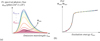 |
Fig. 1 Calculation of PLE spectra from spectrally resolved PL assuming a constant incident photon flux. (a) The PL spectra are measured for different excitation energies Eexc,1 … Eexc,m represented by the various line colors. They are integrated and normalized to the excitation photon flux to provide the PLE spectrum shown in (b). |
3 Methodology
3.1 Sample preparation
The sample under study is described in Figure 2 and fabricated as follows. FTO-coated glass substrates are cleaned, and a compact TiO2 electron transport layer (ETL) is synthesized onto it by atomic layer deposition (ALD). Mesoporous TiO2 is then spin-coated and annealed on top of the c- TiO2 layer before the Glass/FTO/TiO2 substrates are treated with UV-Ozone. The triple-cation perovskite solution consists of a mixture of a solution of CsI in DMSO and another solution of MABr, PbBr2, FAI, and PbI2 of a DMF and DMSO mix. It is deposited onto the substrates by spin coating resulting in a  thin film that is annealed, with an expected bandgap about 1.62 eV [19]. Finally, a 4-FPEAI solution dissolved in IPA at a concentration of 2.5 mg.mL-1 was then spin-coated onto the 3D perovskite and annealed. A reference absorptivity spectrum is measured based on reflection and transmission spectra obtained with an Agilent Cary 5000 spectrometer.
 |
Fig. 2 (a) Structure of the perovskite stack under study, which is illuminated from the perovskite side. (b) Image of reflection of white light illumination onto the sample at 1.53 eV. (c) Areas of interest determined by clustering from the reflection. |
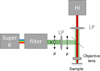 |
Fig. 3 Scheme of the experimental setup. The illumination is filtered by a linear polarizer (LP) before impinging on the sample, forming a homogeneous square with a side length of 400 µm. The emitted PL is collected through the objective and further filtered by the second linear polarizer to attenuate the laser reflection and analyzed by a hyperspectral imager. |
3.2 Experimental setup
As shown in Figure 3, the sample is illuminated with a supercontinuum pulsed laser NKT SuperK with an 80MHz repetition rate and spectrally filtered by a monochromator. The laser is further filtered with Thorlabs FESH800 and FESH850 hard-coated short-pass filters with cut-off wavelengths at 1.55 and 1.46 eV to ensure that no second order is present. The emitted photoluminescence is studied by a hyperspectral imager [20]. To be able to excite the sample with photon energies close to the PL emission, the laser light is filtered out by linear polarization. The laser is homogenized through a square-core optical fiber and is concentrated by the x10 objective onto a 400-micrometer side square, with a constant fluence of 6 × 10¹⁵ photon/cm2/s. Eight different excitation energies between 1.59 and 2.07 eV were used. The experiments are performed by decreasing energy, and one more acquisition is taken at 2.07 eV at the end of the experiment to assess the repeatability of the experiment and monitor the potential effect of light soaking. The sample is placed in a cryostat at −10° C in nitrogen atmosphere and illuminated from the perovskite side. This temperature was chosen to increase the PL signal while remaining close to the room temperature device operation conditions. The measurement was performed after stabilization of the PL spectrum which features a redshift from 1.61 to 1.6 eV during 15 min.
The data collected are spatial images of PL spectra for different excitation energies IPL (x, y, λ, λem) from which we obtain the local PLE (x, y, λexc). This information is completed by estimating the local reflectivity from the hyperspectral images of white light reflection on the sample − denoted Isample (x, y, λ)- and on a mirror − designated by Imirror (x, y, λ):
 (12)
(12)
where the reflectivity of the mirror rmirror (λ) provided by the supplier Thorlabs is taken into account. One can note that the obtained reflectivity value is sensitive to the focus (chromatic aberration) and the angle of the mirror compared to the optical axis of the setup. In addition, due to the collection cone of the objective, it is at best the specular reflectance that is measured, and part of the diffuse light is lost. It is thus assumed that the obtained curve is an approximation of the relative reflectivity, and a correction factor would be required for correcting the optical losses.
For the sake of readability, we further reduced the dimensions to  by clustering the pixels of similar intensities, where i refers to the index of the group of pixels assigned by increasing PL photon flux. The image of reflection at 1.53 eV, shown in Figure 2b, was chosen as a reference for its high contrast and spatial features similar to PL intensity. It is segmented with the K-means algorithm [21]. It allows us to distinguish the five areas of interest displayed in Figure 2c in which the spectra are averaged spatially. This protocol reduces the computing time associated with data fitting while increasing the signal quality but does not refer to a limitation in spatial resolution, estimated in our case to ∼1 μm.
3.3 Simulation of the transient regime
As the PLE experiments are performed with a pulsed laser, a challenge arises for their interpretation: does the approximation of a continuous regime still hold? Indeed, the steady-state hypothesis is at the core of the theoretical framework previously described. It is supported by the short duty cycle (12.5 ns and 80 ps pulses) compared to the charge carrier lifetime expected for perovskite (around 120 ns for a comparable composition [22], and reported in the 40 ns-40 μs range for others [23]). A transient model is used to show that under reasonable assumptions the carrier profile is sufficiently flat, and that the pulsed illumination does not modify the strategy of data analysis.
Drift-diffusion simulations of the PLE experiments are conducted in a transient regime with a one-dimensional homemade code [24]. It calculates the emitted PL from the steps described in Figure 4: for each excitation energy, the generated carriers' profiles are calculated, their transport is obtained by drift-diffusion, and the emitted PL is calculated in-depth and propagated by taking into account reabsorption. For the sake of simplicity, the perovskite sample is modeled as a homogeneous 400 nm-thick slab.
First, the generation profile is modeled from the Beer-Lambert law for an excitation fluence corresponding to the experimental one. The absorption coefficient is estimated from the absorptivity UV-visible spectrometer measurement prolonged below the bandgap energy with a straight exponential tail with an Urbach energy of 30 meV to allow for PL modeling. This value corresponds to the inverse of the logarithmic slope fitted at low energies and is slightly higher than the literature's typical 15-20 meV [25–27]. Second, the drift-diffusion of the generated carriers is computed based on continuity equations for both electrons and holes. They provide the variation of carrier density n in-depth due to transport (drift due to the electric field E and diffusion of coefficient Dn), generation, and recombination rates (resp. G and Reff). For electrons, it reads as:
 (13a)
(13a)
 (13b)
(13b)
These are completed by the Poisson equation and boundary conditions. We set the front recombination velocity at Sfront = 100 cm/s and the back one at Srear = 10 cm/s. This assumption is motivated by the presence of 2D perovskite on top that passivates the sample, and the interface perovskite-TiO2 can be considered well passivated and inducing a low surface recombination velocity. Electrons and holes mobility of 1 cm2/(V.s) were assumed, together with a carrier lifetime of 100ns. At last, the spectral photon flux emitted by PL is calculated by integrating along the depth z Van Roosbroeck-Shockley equation [28], and assuming that reabsorption is described by a term exp(− α (E) z), reading:
 (14)
(14)
Figure 5a shows the carrier concentration profile for a 1.77 eV pulsed excitation as a function of time and depth. This quantity varies only a little during the decay: at the front interface, where its variation is maximal, its amount decreases by 15% before the following pulse. Moreover, the carrier profile is stable with the depth: the variation between the front and rear surfaces is less than 5% for each delay. The situation is then close to the constant profile assumption made to obtain equation (3). For an intrinsic semiconductor, and as stated by equation (10a), PLE intensity is expected to be proportional to the squared density of generated carriers. That is confirmed by the result in Figure 5b. For excitation energies above 1.55 eV, the absorptivity and the square root of PLE differ by less than 2% when scaled at 1.77 eV. This difference is about the setup measurement uncertainty. One possible reason for the mild deviation observed at high excitation wavelengths could be that the density of generated carriers is lower than that at low excitation wavelengths, resulting in an increased role of monomolecular recombination. For instance, at 1.38 eV, the generated carrier density is of the order of 109/cm3, and the assumed intrinsic carrier concentration of 7 × 10⁷/cm3.
Hence, the simulation suggests that the framework leading to a PLE scaling with the squared absorptivity is still valid in our experimental conditions. Yet, a high surface recombination or background doping might cause a difference between the absorptivity obtained by PLE and PL fit.
 |
Fig. 4 Principle of the drift-diffusion model: generation from Beer-Lambert law, drift-diffusion of the carriers, and PL model taking into account reabsorption. |
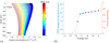 |
Fig. 5 Drift diffusion results. (a) Electron densities for different depths and times after the pulse. (b) Comparison between the square root of PL intensity averaged on the decay and the input absorptivity. The latter is obtained based on transmission and reflection measurements, prolongated with an exponential tail. The ordinates values are scaled to fit at 1.77 eV. |
4 Results
4.1 Luminescence spectral analysis: near gap absorptivity
For a model without interferences and considering constant carrier concentration across the depth, PL emission spectra can be modeled with the generalized Planck's law [29] given in equation (6). It states that the externally emitted spectral photoluminescence photon flux emitted is the product of the absorptivity of the device under test and the blackbody radiation multiplied by carriers' densities. Hence, dividing photoluminescence spectra by the blackbody radiation directly provides relative absorptivity. When normalizing to the photoluminescence photon flux emitted at an arbitrary energy E0, it reads:
 (15)
(15)
One can note that the use of this model is based on strong physical assumptions. Indeed, stating that PL spectra can reflect the absorptivity of the sample implies that [5,6]:
The carrier density profile is approximately uniform (or in the case of negligible reabsorption)
Parasitic absorption is negligible.
Indeed, condition 1 is necessary because a depth dependent carrier profile associated with reabsorption would violate the assumption of formula 6 (ϕem (E)proportional to A(E). Condition 2 establishes that the absorptivity calculated in this way is that of the absorber layer. Yet, this measured absorptivity depends on the experimental conditions. As emphasized by Fassl et al. [30], the PL spectra can be greatly distorted by the escape of photons in total internal reflection due to the roughness of the material. These have lower energies and redshift the measured spectrum, and their share in the collected signal varies depending on the collection optics. With a confocal microscope, their contribution is negligible whereas it is maximum with an integrating sphere.
In addition, the absorptivity obtained locally is affected by the optical properties of neighboring areas. Photons escape laterally away from their emission location [12], which is referred to as photon smearing. As a consequence, it is challenging to retrieve the local absorption coefficient from absorptivity maps. The lateral smearing can be considered negligible in our case, as it occurs on a small length compared to optical resolution and magnification. This mechanism is typically five times the sample thickness (2 μm), which is far smaller than the illumination width (400 μm). If electronic diffusion restricts the spatial resolution of the absorptivity extracted by PLE, which relies on the analysis of charge carrier concentration, it is not detrimental to the absorptivity obtained from equation (14). Instead, it promotes uniformity in carriers, which is advantageous for our model as it helps satisfy condition 1.
The relative absorptivity curves deduced from equation (14) are presented in Figure 6 in different areas of the sample. In this case, the relative absorptivity is normalized by the PL intensity at E0 = 1.68 eV and scaled to the value 1 − R (E0) − T (E0) ∼ 0.64 obtained with the spectrometer. As the reference is measured with an integrating sphere, diffuse reflectance is taken into account. At E0, the absorption length is considered small compared to the thickness of the material and thus the absorptivity is saturating and assumed to be laterally homogeneous. This hypothesis is supported by the uniformity of reflectivity image 1.68 V that owes a standard deviation of 0.0156 and is further supported by the PL image at high energy shown in Figure 7a, which is highly homogeneous. Indeed, the standard deviation of the PL emitted at 1.68ev in the 5 clustering areas of only 1% of the mean intensity. As a consequence of equation (6) considered at high photon energies, this homogeneity suggests a uniform charge carrier density, and thus a uniform ( ). Together with the homogenous reflectance in this energy range and the evaluation of thickness from reflectance in the sub-bandgap range– as presented in the last section- this PL uniformity suggests that τeff, Aexc. and d do not vary much across the sample. By comparison, the normalized standard deviation of PL emission reaches 5% at 1.61 eV, close to the peak energy. The corresponding spatial variations can be seen in Figure 7b, which features a wave-like pattern comparable to the reflectivity.
Figure 7c depicts the ratio of the absorptivity at low energies to the one at higher energies. As the absorptivity is expected to be close to saturation in the high energy range, this image corresponds to a first approximation of the local absorptivity in the [1.55,1.61] eV spectral range. It shows the inhomogeneity of this property below the gap and implies that β varies with the position.
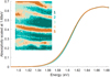 |
Fig. 6 Absorptivity scaled at 1.68 eV in five sample areas which are determined from pixel clustering on the reflection image at 1.53 eV and shown in the inset. They are numbered by increasing intensities − the dark green one has the lowest PL photon flux. |
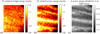 |
Fig. 7 (a)–(b) PL images emitted at high and low energies, averaged in the [1.63,1.68] eV and the [1.55,1.61] eV ranges, respectively, and normalized with respect to their spatial average. They are obtained with the excitation at 2.07 eV. (c) Ratio of the absorptivity image in the low energy range to the one in the high energy range, corresponding in first approximation to the absorptivity between [1.55,1.61] eV. |
4.2 PLE: above-gap absorptivity
The hyperspectral measurements were absolutely calibrated, it is therefore possible to obtain the number of photons emitted locally by integrating the signal spectrally on the whole emission range (mainly contained between 1.44 and 1.75 eV). For excitation energies below 1.84 eV, the reflection of the laser is visible on the spectra at up to 10 nm above the center excitation wavelength. To ensure that this parasitic signal is not taken into account in such cases, the PL spectra are integrated between 1.49 and 1.55 eV. As the PL shape does not change with the excitation energy, they are further rescaled to consider the whole emission spectrum. The corresponding correction factor is estimated with the measurement performed with an excitation energy of 2.06 eV. The obtained result presented in Figure 8 shows an increase in PLE with the excitation energy in all regions of interest, as expected as a result of the growth of the absorptivity.
The intensity of PLE varies depending on the region of interest, which does not necessarily indicate a local change in absorptivity at the excitation energy. Indeed, equations (10a) and (10b) suggest that the PLE scales with  . Thus, the differences in areas could arise from variations in thickness, effective lifetime, or absorptivity (taken either at excitation energy or averaged over the emission spectral range). Additionally, considering only the photons emitted at higher energy in the calculation would lead to a much more homogeneous PLE as can be inferred from Figure 7a. Therefore, variations in PLE intensity from one region to another are dominated by the changes in absorptivity at sub-bandgap energies through β.
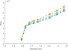 |
Fig. 8 PLE spectra for the different areas of the sample (the color code is similar to previous figures). |
5 Discussion
5.1 Comparing PLE spectroscopy to PL fit
Figure 9 compares the absorptivity values obtained in the two spectral ranges scaled at 1.63 eV and the reference transmission and reflection measurement. The absorptivity obtained by the PL fit and the square root of the PLE both feature a rise close to 1.6 eV. Yet, the three squared PLE measurement points in the PL fit energy range do not scale with it. The 10 nm laser spectral width employed in the experiment corresponds to a minimum horizontal error bar of 20 meV, which could greatly contribute to this misalignment as highlighted by the cross marks indicating this spectral width. However, when taking the rolling average to quickly evaluate the impact of a convolution with the laser spectral width, a window of 30 nm needs to be taken to obtain parallel curves close to the bandgap energy. A change in the injection regime could also contribute to this difference: as shown by equation (9), at low enough absorption, the natural approximation is n << NA. The PLE might scale linearly with the absorptivity in this particular spectral region.
The steep Increase in the absorptivity assessed by PLE happens at energies lower than the one in the reference curve. This is consistent with the ∼0.01 V redshift observed between the initial spectrum and the spectrum taken at the end of the measurement in the same conditions. It highlights the dependence of absorptivity on experimental conditions and the need for its measurement simultaneously with the PL experiment. Moreover, the slope of PLE is steeper than the one of absorptivity. It might be linked to a change in absorptivity between the two measurements induced by material modification under illumination. Indeed, Merdasa et al. [8] have observed a notable impact of excess PbI2 on the slope of both the absorptivity and PLE curves, at comparable energies. This steeper absorptivity might otherwise suggest a reduction in the internal PL quantum yield upon excitation at lower energies. In other words, generating photons further away from the top surface of the sample results in greater non-radiative recombination, which could potentially be attributed to a superior front interface quality as opposed to the rear one. This finding is consistent with the inverse results reported by Bhosale et al. [14], who observed a decrease in the PLE spectrum at higher energies due to increased recombination at the top surface.
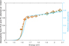 |
Fig. 9 Combination of PL fit and PLE. The dashed lines at high energies represent the curves obtained by PLE. The cross markers associated with them correspond to the spectral width of the excitation laser and provide an idea of the horizontal error bars induced by it. Additional ±2% vertical error bars correspond to the measurement uncertainty from the incident fluence measurement. PL fit is the solid lines and allows for the estimation of absorptivity below 1.7 eV. The scales are adjusted so that the relative absorption averaged on the different areas matches the averaged squared PLE at 1.63 eV. The sky-blue line displays the squared absorptivity obtained from the reference transmission and reflection measurement. |
5.2 Absorptivity from PL fit − an outlook through reflection measurements
Fitting the absorptivity from the PL requires a model for the absorption coefficient and for its link to the absorptivity. It offers a possible way to retrieve the absorption coefficient multiplied by the absorber thickness and separate these quantities from the charge carrier density. In this paragraph, such a strategy is employed with our data in order to scale the absorptivity and get closer to the determination of the absorption coefficient.
It Is assumed that the absorptivity of a thick sample is given by the Beer-Lambert law and can be written as A (λ) = 1 − exp(− α (λ) d). The reflection is neglected to assess what can be obtained from PL itself. We further fit the absorption coefficient with Katahara model [31], which expresses α as a function of a scaling constant α0, the bandgap energy Eg, a characteristic tail energy γ, and an exponent θ: an ideal absorption coefficient expressed as  is convoluted to the following sub-bandgap tail states density
  where N is a normalization factor. Spectral fit is performed with the laser excitation energy set at 2.07 eV to ensure the absence of a parasitic peak on the spectrum coming from the illumination. The results are presented in Figure 10 in different areas of the sample, and the associated values are provided in Table 1. Our data reasonably fit with θ = 1.5. The fitted band tails of the different areas of the sample are very similar and suggest that the absorption coefficient of the material is homogeneous for energies below the gap. Yet, this approach still strongly relies on the optical model and cannot disentangle the absorption scaling factor α0 from the thickness of the sample. We explore the data treatment of white light reflection to fit this second quantity.
The results of the reflectivity assessment presented in Figure 11b show a similar trend for all areas: the reflectivity is stable above 1.64 eV, whereas for energies below the absorption threshold of perovskite, interferences can be seen. The reflectivity at high energy is quite uniform, with a relative variation of 14% yet resulting in changes of 1-R of less than 2%, which supports the above scaling of the absorptivity at 1.68 eV. The reference reflectivity at this energy is 0.17, of the same order of magnitude. By comparison with the PL spectra in the corresponding areas shown in Figure 11a, it can be inferred that the variation in the reflectivity is the main reason for the variation of the PL spectrum. This calls into question the results of the absorptivity fit, as the photoluminescence shape is greatly impacted by the reflectivity in the sub-bandgap range. It is likely that α0d does not change so significantly and that the sample presents only minor topological changes.
Additionally, the interference patterns suggest that Region 1 is thinner than Region 5: the peak energy of the reflectivity shifts corresponds to 42 nm towards the higher wavelengths. The change in thickness compatible with this shift and the known optical index of perovskites is in the range of dozens of nanometers. This observation goes against the trend observed for the above fit of α0d in the Section 4.2 model that does not include interferences. This observation emphasizes the need for better optical models compared to the ones typically used for fitting the photoluminescence spectra. It also stresses the importance of considering local reflectivity rather than using spatially averaged values, as the latter approach is unlikely to provide a meaningful fit for the absorption edge. Both considerations are necessary for a robust quantitative absorption coefficient and effective lifetime mapping.
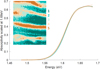 |
Fig. 10 Fit of the absorptivity normalized at peak energy (dashed lines) with the Katahara model (solid lines) in the regions of interest. |
Katahara fit results in the different areas.
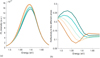 |
Fig. 11 Comparison between (a) the PL spectra for a 600 nm excitation and (b) reflectivity of the sample in the different areas assessed using white light reflection through equation (15). |
6 Conclusion
We have presented a proof of principle of a local absorptivity measurement resolved spatially at the micrometer scale through hyperspectral photoluminescence excitation imaging. We confirmed by simulation that the use of a pulsed laser should not hinder the extraction of absorptivity from PLE in our case. The relative absorptivity was obtained close to the bandgap energy by analyzing the emission spectrum and in a complementary range, at energies above the gap, by PLE, therefore enabling to cover of all the absorption ranges relevant to solar cells. As the charge carrier densities scale with both the absorbed photon flux and an effective lifetime, calibrated PLE on its own cannot completely disentangle the contribution from local absorptivity and local recombination properties. A further quantitative measurement is necessary to scale the measured absorptivity locally, such as UV-visible spectroscopy. Nevertheless, the analysis of the PL emission ratio at different wavelengths suggests that the variations of PL intensity observed for our sample mainly come from inhomogeneity in the sub-bandgap absorptivity and that electronic properties are rather uniform. Furthermore, completing the PLE by a spatial reflection measurement provides insight into the optical and structural properties of the device, and can help improve the optical model to be used. Notably, it was found that the spatial variations of the absorptivity below the gap are most likely caused by the non-uniformity of the absorber thickness. The study also stressed that reflectivity can significantly impact the results of the absorption coefficient fit, also on a local scale, and the optical model needs to be improved to obtain an accurate quantitative assessment of the absorber properties.
We thank Daniel Micha for the scientific discussion around this topic and Emilie Raoult for providing the optical indices used in this study. This project has been supported by the ANRT CIFRE convention N° 2019/0780, and by the program CHARMING of IPVF.
Author contribution statement
Marie Legrand performed the data acquisition and treatment and wrote the manuscript. Baptiste Bérenguier created the simulation tool. Baptiste Bérenguier and Marie Legrand carried out the calculations. Thomas Campos synthesized the perovskite sample. Daniel Ory and Jean-François Guillemoles provided critical feedback and contributed to shaping this research work.
References
- D.C. Look, J.H. Leach, On the accurate determination of absorption coefficient from reflectanceand transmittance measurements: application to Fe-doped GaN, J. Vac. Sci. Technol. B, Nanotechnol. Microelectron.: Mater. Process. Meas. Phenom. 34, 04J105 (2016) [Google Scholar]
- P. Pearce, RayFlare: flexible optical modelling of solar cells, JOSS 6, 3460 (2021) [CrossRef] [Google Scholar]
- M. Seitz et al., Mapping the trap-state landscape in 2D metal‐halide perovskites using transient photoluminescence microscopy, Adv. Optical Mater. 9, 2001875 (2021) [Google Scholar]
- R. Bhattacharya, B. Pal, B. Bansal, On conversion of luminescence into absorption and the van Roosbroeck-Shockley relation, Appl. Phys. Lett. 100, 222103 (2012) [CrossRef] [Google Scholar]
- E. Daub, P. Würfel, Ultralow values of the absorption coefficient of Si obtained from luminescence, Phys. Rev. Lett. 74, 1020 (1995) [CrossRef] [PubMed] [Google Scholar]
- C. Barugkin et al., Ultralow absorption coefficient and temperature dependence of radiative recombination of CH3NH3PbI3 perovskite from photoluminescence, J. Phys. Chem. Lett. 6, 767 (2015) [CrossRef] [Google Scholar]
- T. Trupke, E. Daub, P. Würfel, Absorptivity of silicon solar cells obtained from luminescence, Sol. Energy Mater. Sol. Cells 53, 103 (1998) [CrossRef] [Google Scholar]
- A. Merdasa et al., Impact of excess lead iodide on the recombination kinetics in metal halide perovskites, ACS Energy Lett. 4, 1370 (2019) [CrossRef] [Google Scholar]
- D. Berdebes et al., Photoluminescence excitation spectroscopy for in-line optical characterization of crystalline solar cells, IEEE J. Photovoltaics 3, 1342 (2013) [CrossRef] [Google Scholar]
- J. Jimenez, J.W. Tomm, Photoluminescence (PL) techniques, in Spectroscopic Analysis of Optoelectronic Semiconductors (Springer International Publishing, 2016), Vol. 202, pp. 143–211 [CrossRef] [Google Scholar]
- E.K. Grubbs, J. Moore, P.A. Bermel, Photoluminescence excitation spectroscopy characterization of surface and bulk quality for early-stage potential of material systems, in 2019 IEEE 46th Photovoltaic Specialists Conference (PVSC) (IEEE, 2019), pp. 0377–0381. doi:10.1109/PV SC40753. 2019.8980637 [Google Scholar]
- H.T. Nguyen et al., Spatially and spectrally resolved absorptivity: new approach for degradation studies in perovskite and perovskite/silicon tandem solar cells, Adv. Energy Mater. 10, 1902901 (2020) [CrossRef] [Google Scholar]
- M.K. Juhl, T. Trupke, M. Abbott, B. Mitchell, Spatially resolved absorptance of silicon wafers from photoluminescence imaging, IEEE J. Photovoltaics 5, 1840 (2015) [CrossRef] [Google Scholar]
- J.S. Bhosale, J.E. Moore, X. Wang, P. Bermel, M.S. Lundstrom, Steady-state photoluminescent excitation characterization of semiconductor carrier recombination, Rev. Sci. Instrum. 87, 013104 (2016) [CrossRef] [PubMed] [Google Scholar]
- X. Wang et al., Photovoltaic material characterization with steady state and transient photoluminescence, IEEE J. Photovoltaics 5, 282 (2015) [CrossRef] [Google Scholar]
- R.C. Miller, A.C. Gossard, G.D. Sanders, Y.-C. Chang, J.N. Schulman, New evidence of extensive valence-band mixing in GaAs quantum wells through excitation photoluminescence studies, Phys. Rev. B 32, 8452 (1985) [CrossRef] [PubMed] [Google Scholar]
- M.C. DeLong et al., Photoluminescence, photoluminescence excitation, and resonant Raman spectroscopy of disordered and ordered Ga0.52 In0.48 P, J. Appl. Phys. 73, 5163 (1993) [CrossRef] [Google Scholar]
- X. Wang et al., Valence band splitting in wurtzite InGaAs nanoneedles studied by photoluminescence excitation spectroscopy, ACS Nano 8, 11440 (2014) [CrossRef] [PubMed] [Google Scholar]
- T. Campos et al., Unraveling the formation mechanism of the 2D/3D perovskite heterostructure for perovskite solar cells using multi-method characterization, J. Phys. Chem. C 126, 13527 (2022) [CrossRef] [Google Scholar]
- A. Delamarre, Characterization of solar cells using electroluminescence and photoluminescence hyperspectral images, J. Photon. Energy 2, 027004 (2012) [CrossRef] [Google Scholar]
- S. Lloyd, Least squares quantization in PCM, IEEE Trans. Inform. Theory 28, 129 (1982) [CrossRef] [Google Scholar]
- S. Cacovich et al., In-depth chemical and optoelectronic analysis of triple-cation perovskite thin films by combining XPS profiling and PL imaging, ACS Appl. Mater. Interfaces 14, 34228 (2022) [CrossRef] [PubMed] [Google Scholar]
- J.Y. Kim, J.-W. Lee, H.S. Jung, H. Shin, N.-G. Park, High-efficiency perovskite solar cells, Chem. Rev. 120, 7867 (2020) [CrossRef] [PubMed] [Google Scholar]
- B. Bérenguier et al., Defects characterization in thin films photovoltaics materials by correlated high-frequency modulated and time resolved photoluminescence: an application to Cu(In,Ga)Se2, Thin Solid Films 669, 520 (2019) [CrossRef] [Google Scholar]
- S. De Wolf et al., Organometallic halide perovskites: sharp optical absorption edge and its relation to photovoltaic performance, J. Phys. Chem. Lett. 5, 1035 (2014) [CrossRef] [Google Scholar]
- B.T. Van Gorkom, T.P.A. Van Der Pol, K. Datta, M.M. Wienk, R.A.J. Janssen, Revealing defective interfaces in perovskite solar cells from highly sensitive sub-bandgap photocurrent spectroscopy using optical cavities, Nat. Commun. 13, 349 (2022) [CrossRef] [Google Scholar]
- S. Cacovich et al., Imaging and quantifying non-radiative losses at 23% efficient inverted perovskite solar cells interfaces, Nat. Commun. 13, 2868 (2022) [CrossRef] [Google Scholar]
- W. van Roosbroeck, W. Shockley, Photon-radiative recombination of electrons and holes in germanium, Phys. Rev. 94, 1558 (1954) [CrossRef] [Google Scholar]
- P. Würfel, S. Finkbeiner, E. Daub, Generalized Planck's radiation law for luminescence via indirect transitions, Appl. Phys. A 60, 67 (1995) [CrossRef] [Google Scholar]
- P. Fassl et al., Revealing the internal luminescence quantum efficiency of perovskite films via accurate quantification of photon recycling, Matter 4, 1391 (2021) [CrossRef] [Google Scholar]
- J.K. Katahara, H.W. Hillhouse, Quasi-Fermi level splitting and sub-bandgap absorptivity from semiconductor photoluminescence, J. Appl. Phys. 116, 173504 (2014) [CrossRef] [Google Scholar]
Cite this article as: Marie Legrand, Baptiste Bérenguier, Thomas Campos, Daniel Ory, Jean-François Guillemoles, Investigations on photovoltaic material absorptivity using hyperspectral photoluminescence excitation imaging, EPJ Photovoltaics 14, 40 (2023)
All Tables
All Figures
|
Fig. 1 Calculation of PLE spectra from spectrally resolved PL assuming a constant incident photon flux. (a) The PL spectra are measured for different excitation energies Eexc,1 … Eexc,m represented by the various line colors. They are integrated and normalized to the excitation photon flux to provide the PLE spectrum shown in (b). |
| In the text | |
|
Fig. 2 (a) Structure of the perovskite stack under study, which is illuminated from the perovskite side. (b) Image of reflection of white light illumination onto the sample at 1.53 eV. (c) Areas of interest determined by clustering from the reflection. |
| In the text | |
|
Fig. 3 Scheme of the experimental setup. The illumination is filtered by a linear polarizer (LP) before impinging on the sample, forming a homogeneous square with a side length of 400 µm. The emitted PL is collected through the objective and further filtered by the second linear polarizer to attenuate the laser reflection and analyzed by a hyperspectral imager. |
| In the text | |
|
Fig. 4 Principle of the drift-diffusion model: generation from Beer-Lambert law, drift-diffusion of the carriers, and PL model taking into account reabsorption. |
| In the text | |
|
Fig. 5 Drift diffusion results. (a) Electron densities for different depths and times after the pulse. (b) Comparison between the square root of PL intensity averaged on the decay and the input absorptivity. The latter is obtained based on transmission and reflection measurements, prolongated with an exponential tail. The ordinates values are scaled to fit at 1.77 eV. |
| In the text | |
|
Fig. 6 Absorptivity scaled at 1.68 eV in five sample areas which are determined from pixel clustering on the reflection image at 1.53 eV and shown in the inset. They are numbered by increasing intensities − the dark green one has the lowest PL photon flux. |
| In the text | |
|
Fig. 7 (a)–(b) PL images emitted at high and low energies, averaged in the [1.63,1.68] eV and the [1.55,1.61] eV ranges, respectively, and normalized with respect to their spatial average. They are obtained with the excitation at 2.07 eV. (c) Ratio of the absorptivity image in the low energy range to the one in the high energy range, corresponding in first approximation to the absorptivity between [1.55,1.61] eV. |
| In the text | |
|
Fig. 8 PLE spectra for the different areas of the sample (the color code is similar to previous figures). |
| In the text | |
|
Fig. 9 Combination of PL fit and PLE. The dashed lines at high energies represent the curves obtained by PLE. The cross markers associated with them correspond to the spectral width of the excitation laser and provide an idea of the horizontal error bars induced by it. Additional ±2% vertical error bars correspond to the measurement uncertainty from the incident fluence measurement. PL fit is the solid lines and allows for the estimation of absorptivity below 1.7 eV. The scales are adjusted so that the relative absorption averaged on the different areas matches the averaged squared PLE at 1.63 eV. The sky-blue line displays the squared absorptivity obtained from the reference transmission and reflection measurement. |
| In the text | |
|
Fig. 10 Fit of the absorptivity normalized at peak energy (dashed lines) with the Katahara model (solid lines) in the regions of interest. |
| In the text | |
|
Fig. 11 Comparison between (a) the PL spectra for a 600 nm excitation and (b) reflectivity of the sample in the different areas assessed using white light reflection through equation (15). |
| In the text | |
Current usage metrics show cumulative count of Article Views (full-text article views including HTML views, PDF and ePub downloads, according to the available data) and Abstracts Views on Vision4Press platform.
Data correspond to usage on the plateform after 2015. The current usage metrics is available 48-96 hours after online publication and is updated daily on week days.
Initial download of the metrics may take a while.