


| Issue |
EPJ Photovolt.
Volume 17, 2026
Special Issue on ‘EU PVSEC 2025: State of the Art and Developments in Photovoltaics', edited by Robert Kenny and Carlos del Cañizo
|
|
|---|---|---|
| Article Number | 23 | |
| Number of page(s) | 15 | |
| DOI | https://doi.org/10.1051/epjpv/2026015 | |
| Published online | 22 June 2026 | |
https://doi.org/10.1051/epjpv/2026015
Original Article
Modeling partial shading at the cell level on photovoltaic modules
1
UCP, ENSTA, Institut Polytechnique de Paris, 828 Boulevard des Maréchaux, 91120 Palaiseau, France
2
EPFL, PV-Lab, Maladière 71b, 2000 Neuchâtel, Switzerland
3
CSEM, Sustainable Energy Center, Jaquet-Droz 1, 2000 Neuchâtel, Switzerland
* e-mail: This email address is being protected from spambots. You need JavaScript enabled to view it.
Received:
1
October
2025
Accepted:
24
April
2026
Published online: 22 June 2026
Abstract
The growing integration of photovoltaic (PV) systems into complex environments—such as rooftops, façades, and vehicles—has introduced new shading patterns and the need for accurate performance modeling under these partial shading conditions. In particular, building-integrated photovoltaics (BIPV) are often subject to thin shadows from nearby building components, vegetation, or infrastructure. These shadings can impact only portions of individual cells, leading to inhomogeneous irradiances that are difficult to capture with conventional simulation tools. A few commercial tools consider the impact of near shading losses on photovoltaic arrays, a well-documented example being PVsyst. PVsyst incorporates a more sophisticated approach using four empirically derived I-V curve templates based on the number of shaded corners per sub-module, but the core logic remains: if at least one corner of a sub-module intersects a shadow, it is treated as electrically shaded. This assumption is valid for large open-rack systems with large shadows. The choice of points to check for shadow intersection could however be improved for thin shadows by considering partial shading at the cell level. This work presents a shadow modeling approach based on vertex projection, and the shadow positions were experimentally validated against photographs of shadows cast on an outdoor BIPV module in Neuchâtel, Switzerland. The near shading simulation is done at the cell level, and several strategies for selecting points to check for shadow intersection are compared to determine the shaded fraction and shading-adjusted plane-of-array irradiance of each cell. This irradiance is calculated by summing the diffuse plane-of-array irradiance and the direct plane-of-array irradiance adjusted for the shaded fraction. Compared with a conservative full-shading baseline, the cell-level model which captures partial cell shading may predict about 2% lower annual irradiance losses for a 25 cm shadow and even more for thinner shadows. At sufficient resolution, the model avoids missing thin shadows entirely—a key limitation of the submodule-level approach. The algorithm scales efficiently at low resolutions, simulating a full year of hourly cell irradiance data in about 17 s for a 40-cell module at 2 × 2 to 5 × 5 points per cell, and about 25 s for 1200 cells at 3 × 3 resolution.
Key words: Partial Shading / photovoltaic performance modeling / vertex projection / cell-level simulation / BIPV
Publisher note: The affiliation numbers assigned to the authors were corrected on 30 June 2026.
© J.-P. Calin et al., Published by EDP Sciences, 2026
 This is an Open Access article distributed under the terms of the Creative Commons Attribution License (https://creativecommons.org/licenses/by/4.0), which permits unrestricted use, distribution, and reproduction in any medium, provided the original work is properly cited.
1 Introduction
The increasing demand for renewable energy sources has expanded the adoption of photovoltaic (PV) systems across diverse sectors, including buildings, infrastructure, transportation, and agriculture. As PV technologies become increasingly integrated into urban and architectural environments — particularly through applications like building-integrated photovoltaics (BIPV) and vehicle-integrated photovoltaics (VIPV) — different shading patterns are being observed on these integrated PV systems. This opens the door to reconsider our shadow modeling strategies to more accurately model performance under these new partial shading conditions. Shadows cast by nearby objects like chimneys, dormers, railings, trees, or adjacent buildings can significantly reduce energy yield, particularly in dense or irregular environments. These shading effects are often highly localized, affecting only parts of individual cells, and their impact on electrical performance is nonlinear and configuration-dependent. Thus, complex geometries and urban contexts introduce new needs when accounting for near shading losses to make an accurate performance prediction.
The concept of “near shading” was introduced by Mermoud et al. [1] in the development of PVsyst, which remains a widely used simulation tool in the PV industry. PVsyst uses the sub-module as the basic unit for computing the IV curve. As the cells in a sub-module are connected in series, the number of shaded cells in a sub-module does not impact the IV curve. Depending on the number of corners shaded, the sub-module IV curve is modeled by one of four empirically derived IV curve templates. These templates do not scale irradiance linearly with the number of corners, but reflect the fact that heavy losses could occur even if only one corner of the sub-module is shaded, being that a whole cell could be shaded. This essentially means that the sub-module is considered fully shaded from an electrical perspective if at least one corner of a sub-module intersects a shadow. While this approach enables fast, empirically-backed simulations for large PV systems with large shadows, it is perhaps less suited to small systems with thin shadows. If the shadows are large and tend to cover at least one corner as they pass over the sub-modules, the approach is conservative and provides an upper limit on near shading losses. Yet, if the shadows tend to be thinner than the submodule, we could miss them as they pass over if we are checking only the corners of each sub-module.
A logical way to improve this is to model shading at the cell level, whereby we can account for the shading of individual cells, even partial shading on individual cells. Checking more points for shadow intersection will decrease the likelihood of missing shadows thinner than a submodule. Checking several points per cell will enable us to account for the partial shading of cells, reducing the chance that we overestimate shading losses from shadows thinner than a cell.
Recent research has sought to improve the spatial resolution and physical realism of shading models. De Sá et al. [2] proposed a rasterization-based algorithm that projects shadows from convex obstructions onto PV arrays using solar geometry and convex hull logic. This algorithm supports high spatial resolution and can, in principle, compute irradiance at the cell level, but the model in the study assumes uniform irradiance across each module and does not account for internal cell interconnections.
Mikofski et al. [3] introduced SolarFarmer, a performance model that uses a hemicube-based back-tracing method to simulate shading and mismatch. With this approach, irradiance is calculated at a specified number of target points on the array. The sampling point resolution in the study was varied from one point per module to one point per cell. Increasing from one point per module to five points per sub-module resulted in a relative 17% reduction in the annual prediction error. Little further improvement was observed at one point per cell, as the error with respect to measurements remained at 0.5%. The SolarFarmer model was validated in [3] on regular, broad area shadows from a large flat-top building near the array. As noted in [4], more validation against real data under different shading configurations is needed to determine if the error is a consistent bias or linked to the specific shading configuration in the study. The literature on shading modeling at the cell level is very scarce and in need of investigation into the impact of resolution on irregular, more localized shadow configurations.
Meyers et al. [4] developed a fast shading model (FSM) to predict the effective irradiance on each cell computed by a simplified 5-parameter (S5P) model. The neural network model was trained through statistical analysis of hundreds of thousands of shading scenarios and validated on a real PV system with shading from three adjacent pipes. The study demonstrated a cell-level shading simulation with a dramatic runtime reduction using a simplified neural network compared to a physics-based approach, at the expense of higher prediction uncertainty. The shadows were projected onto the 3D system to produce an image, from which the shaded area was extracted to compute cell effective irradiance.
For comparison, Meyers et al. [4] considered two common methods for determining shading losses: the shading impact factor (SIF) model used by the California Energy Commission (CEC), and a simplified linear model that assumes power losses equal to irradiance losses, consistent with the “solar access” values provided by tools like the Solmetric SunEye. The SIF and linear models tend to under-predict real power losses due to shading, whereas the S5P and FSM models tend to over-predict them, especially at the tails of the day when long, narrow shadows are cast on the modules in the test configuration. The FSM predicted the S5P model outputs very accurately, with the differences well within the 95% confidence interval, on the test configuration in the study. However, the authors pointed out that FSM could predict higher losses than S5P on other system or shade configurations. Therefore, more work is needed to determine the discrepancy between the measurements and S5P results.
The goal of this work is to develop a physics-based near shading model to compute the shading-adjusted plane-of-array irradiance on each cell in a PV module under conditions of thin shadows. We are interested in finding a potential improvement in accuracy while limiting the increase in computation time. To this effect, the key focus is to vary the logic for sampling points to check for shadow intersection. Sampling more points may enable quantifying shading losses more accurately, at the cost of added computation time, which will also be assessed.
2 Material and methods
2.1 Three-step framework
In this work, we present a framework for near shading analysis at the cell level. Similar to current near shading methods, this approach consists of three main steps. The first step is shadow modeling, where the shadow is projected onto the ground plane using a vertex projection approach. Second, the shaded fraction of each cell or sub-module is estimated by checking a sample of points for shadow intersection. Third, the shading-adjusted plane-of-array irradiance on each sub-module or cell is modeled using the simulated shaded fractions and ground irradiance data.
2.2 Shadow modeling
The first two steps of this framework were initially implemented using a 3D shadow modeling method, described in the following section. Because this approach becomes computationally demanding at high resolutions, we introduced several modifications to reduce the simulation time and developed a faster 2D vertex projection method, which is presented after the 3D method. To contextualize the runtime comparisons that follow, all measurements reported in this manuscript were obtained using a workstation with an AMD Ryzen 7 Pro 5845 processor (8 cores, 3.40 GHz) and 80 GB DDR4‑3200 RAM.
2.2.1 3D method
The 3D vertex projection method was inspired by the algorithm proposed by de Sá et al. [2], which models shadows from nearby obstructions using geometric projections and convexity principles. First, the spatial coordinates of the modules and nearby objects are computed in the Cartesian space. An example model configuration for the experimental setup in this study is illustrated in Figure 1a. The method then calculates the solar position, meaning the solar azimuth and apparent elevation angles, using astronomical equations that account for the Earth's elliptical orbit and axial tilt and atmospheric refraction [5]. These angles define the direction of incident sunlight and are used to project the vertices of 3D obstructions onto the ground plane. The projection is only performed during daytime, when the solar elevation angle is above zero.
To reduce computational complexity, the algorithm assumes that shadows cast by convex objects are themselves convex. Thus, only the outermost vertices, called the convex hull, of each obstruction are projected onto the ground plane. These vertices are shown in blue in Figure 1b, and their projections onto the ground plane in green. The union of these vertices and their projections defines the total 3D shadow region, as shown in Figure 1c.
Once the 3D shadow region is defined, a rasterization process is applied to determine which fraction of the PV cell is shaded. The module surface is discretized into a grid of points, the corners or centroids of sub-modules, cells, or sub-cells, each of which is tested for inclusion within the shadow region. A point is considered shaded if its inclusion does not alter the convex hull of the shadow region, following the logic described in de Sá et al. [2]. Because the number of points on the grid can be specified, the rasterization approach allows us to tune the spatial resolution according to the desired computational speed and spatial accuracy. An example cell shadow raster with 40 × 40 resolution is shown in Figure 1d, and the module shadow raster in Figure 1e.
As the spatial resolution of the raster increases, the computational cost can become a practical constraint. The cell shadow rasterization becomes the most time-intensive component of the original 3D approach because a 3D convex hull has to be computed for every point on the module plane that is checked for shadow intersection. This operation takes about 1 millisecond per point, so checking 64,000 points across 40 cells at 40 × 40 points per cell requires at least 64 s per solar position. Including all other steps in the 3D method, the runtime is around 78 s per solar position. Because the near shading simulation is used to estimate annual losses over a full year of hourly data, about half of which are daylight hours, the total runtime would be roughly 95 h.
To make the simulation time manageable, we introduced a simplification that reduces the number of points checked per cell. We observed that most cells remain fully unshaded, even during hours when the shadow passes over the module, because the shadow is much narrower than the module width. This means that unnecessary computation can be avoided at higher resolutions (3 × 3 and above) by first checking only the corners of each cell. If all four corners intersect the shadow, the cell is assumed fully shaded; if none of the corners intersect the shadow, the cell is treated as unshaded. At 40 × 40 resolution, the runtime decreases in proportion to the number of cells skipped by this check, from about 2 s per cell to about 2 s per partially shaded cell. In our case, where only about 10% of cells were partially shaded on average over all daylight hours in the year, the simplified 3D method reduces the annual simulation time nearly ten-fold at 40 × 40 resolution, from an estimated 95 h to a measured 9.93 h.
However, this logic is only appropriate if the total number of points sampled per cell is more than the four corners; clearly it would not reduce computation at resolutions of 1 × 1 or 2 × 2. It also only makes sense if the shadows cast on the module are at least as wide as the cells, otherwise the likelihood of missing thinner shadows would increase. The simplification is valid for our experimental configuration, but for thinner shadows, more points should be used along the edges of the cells in order to mitigate the risk of missing shadows.
A remaining limitation of the 3D approach is that shadow intersection must still be evaluated point by point, an operation which cannot be accelerated through vectorized computation, as will be discussed. To improve computational efficiency, we replace the 3D convex hull check with a 2D point-in-polygon test, which forms the basis of the 2D method described next.
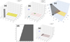 |
Fig. 1 3D Vertex projection approach: (a) model configuration, (b) vertices projected on ground plane, (c) 3D shaded region, (d) cell shadow raster, (e) module shadow. |
2.2.2 2D method
The 2D approach, illustrated in Figure 2, begins with the same 3D model configuration (Fig. 2a). The shadow modeling procedure also begins with projecting obstacle vertices onto the ground plane (Fig. 2b), but instead of a 3D convex hull, the shadow is modeled as a 2D polygon on the ground plane (Fig. 2c). To compute the shaded fraction of each cell or sub-module, its corners are projected onto the ground plane (Fig. 2d), forming a quadrilateral that is subdivided at the chosen resolution to obtain sample points (Fig. 2e shows a resolution of 2 × 2 points per cell). These sample points are then checked for shadow intersection using a point-in-polygon test (Fig. 2f).
In our first implementation of this 2D approach, the most time-intensive operation was computing the coordinates of the sampled points on the ground plane (Fig. 2e). The projected corners of each cell form a rhombus, which we subdivide parametrically using bilinear interpolation between the four corner points. For a sampling resolution of N × N points per cell, this produces N2 sample points. Initially, the bilinear interpolation used to generate these sample points was performed inside a loop, which causes the runtime to scale quadratically with resolution N (blue curve in Fig. 3). We replaced the loop with a more efficient, vectorized computation applied once per cell, which significantly reduces the runtime growth (green curve). A further reduction across all resolutions was made by running the operation once across all cells (violet curve). Similarly, we vectorized and combined the two vertex projection steps (Figs. 2b and 2d) so the computation is performed once for all obstacle vertices and cell points (grey curve).
Figure 3 shows the runtime of the 3D and 2D methods at different resolutions. The simplified 3D method (yellow curve, with 10% of cells partially shaded) is faster than the original 3D method (orange curve) at resolutions of 3 × 3 and above, although its runtime depends on the number of partially shaded cells, which varies with solar position. The 2D method is significantly faster than both 3D approaches, even before vectorization (blue curve). After vectorization, the 2D method (grey curve) shows further reductions in runtime and a slower increase with resolution, running in about 16 ms per solar position at 40 × 40 resolution and about 5 ms at resolutions between 1 × 1 and 10 × 10. As we discuss further in the results section, this reduces the total simulation time over 1-yr hourly data to the order of seconds.
This 2D projection approach, however, relies on an assumption not required by the 3D method. It assumes a cell point is shaded whenever its projection lies inside the shadow polygon. Geometrically, this means that the line passing through the cell point and aligned with the sun vector must also pass through the obstacle. This assumption holds when the obstacle is truly positioned between the sun and the module. However, if the obstacle lies behind the module along the same projection line—for example, when the module casts a shadow onto the obstacle rather than the obstacle casting a shadow onto the module—it can produce false shadows. In our configuration, with the obstacle located south of the PV module, no such false shadows occurred over the year. Nonetheless, this remains an important limitation of the 2D method. A possible solution would be to filter out obstacles from the analysis during times or solar positions when their location makes them unlikely to cast a shadow on the module. This could also be addressed by computing a shadow depth map and comparing the depth of projected points to the shadow depth.
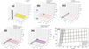 |
Fig. 2 2D approach: (a) model configuration, (b) obstacle vertices projected onto ground plane, (c) 2D shadow polygon, (d) cell corners projected onto ground plane, (e) points sampled at desired resolution on ground plane, (f) point-in-polygon test for shadow intersection. |
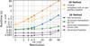 |
Fig. 3 Runtime per solar position of the 3D and 2D methods at different resolutions. |
2.3 Shadow detection logic
With the shadow geometry established through the projection methods described above, the second step of the framework is to determine the shaded fraction of individual sub-modules or cells, based on a set of sampled points to check for shadow intersection. We select points to check for shadow intersection using several strategies, at the sub-module level or the cell level, and using corners or centroids. These approaches are compared on the example in Figure 4. A dark grey shadow covers much of the top row of cells in a sub-module consisting of 6 square cells. The red circles represent the points to be checked for shadow intersection.
The rows of Figure 4 compare the corner-based and centroid-based logic. Corner-based intersection is defined as follows: a sub-module, cell, or sub-cell is considered shaded if at least one of its corners intersects the shadow. Centroid-based intersection is defined as follows: a cell or sub-cell is considered shaded only if its centroid lies within the shadow polygon. This method requires only one point per sub-module, cell, or sub-cell, compared with four points in the corners-based approach.
The columns in the figure contrast the resolutions of sampling points at the sub-module, cell, and sub-cell level. Submodule-level modeling assumes the sub-module is shaded from an electrical standpoint if at least one sampled point intersects a shadow. Cell-level modeling assigns unique irradiance values to each cell, by computing the shaded fraction of each cell. At 1 × 1 resolution, each cell is considered either fully shaded (shaded fraction equals 1) or not at all shaded (0). By increasing the resolution, we can more precisely determine the shaded fraction of each cell.
The corner-based, sub-module level approach presented on the top left in the figure was inspired by PVsyst’s module layout tool, which uses a more elaborate method to construct array I-V curves based on sub-module shading. In PVsyst, the sub-module I-V curve is modeled using an experimentally derived template based on the number of corners shaded per sub-module, where even the template for one shaded corner reflects the fact that heavy shading losses could occur as a cell may be fully shaded. Similarly, the sub-module level model in this work assigns a shaded fraction of 1 to a sub-module if any corner intersects the shadow; otherwise, the shaded fraction is 0.
 |
Fig. 4 Comparison of methods to determine which points to check for shadow intersection. Corner-based (top) vs. centroid-based (bottom) intersection logic. Point sampling at submodule-level (left) vs. cell-level at resolution 1 × 1 (center) and 2 × 2 (right). |
2.4 Irradiance modeling
The third step of the framework models the irradiance on each sub-module or cell based on its shaded fraction and the measured irradiance components. Irradiance on each cell or sub-module is computed using an isotropic sky model [6], where the global plane-of-array irradiance (GPOA), in the absence of near shading, is calculated according to [6] using the pvlib python library [5]:
 (1)
(1)
where Gbeam is the direct (beam) irradiance component, Gsky diffuse is the sky diffuse component, and Gground is the ground-reflected diffuse component.
The direct irradiance in the plane-of-array is:
 (2)
(2)
where DNI is the direct normal irradiance and θ is the angle of incidence of the solar rays on the module surface.
The diffuse sky irradiance in the plane-of-array, according to the isotropic sky model [6,7] is:
 (3)
(3)
where DHI is the diffuse horizontal irradiance and β is the module tilt angle (15° in this study).
The ground-reflected diffuse irradiance in the plane-of-array [6] is:
 (4)
(4)
where GHI is the global horizontal irradiance and ρ is the ground surface albedo, assumed to be 0.25.
In the cell-level approach, the irradiance on each cell is calculated from its shaded fraction and the direct and diffuse irradiance components. The direct component is assumed to reach only the unshaded surface of the cell, whereas the diffuse components reach the entire cell surface:
 (5)
(5)
where Gcell is the cell irradiance and χ is the shaded fraction of the cell. Equivalently, in terms of GPOA:
 (6)
(6)
The same expression is used in the submodule-level approach, where χ represents the shaded fraction of the sub-module and Gsubmodule replaces Gcell.
As input to the irradiance model, we used hourly typical meteorological year (TMY) data from PVGIS [8], which provides DNI, DHI, and GHI. We also applied the model to ground measurements, including GPOA, DHI, and GHI recorded at 3 min intervals by three pyranometers on a weather monitoring station located a few meters from the experiment. The diffuse plane-of-array irradiance components Gsky diffuse and Gground were modeled from measured DHI and GHI using equations (3) and (4). From these values and the measured GPOA, the direct plane-of-array irradiance Gbeam was computed using equation (1). These irradiance components and the modeled shaded fraction χ were then substituted into equation (5) to obtain the cell- and submodule-level irradiance.
2.5 Irradiance losses
To quantify the loss of irradiance on the module due to near shading, we consider that module current is limited by the sub-module or cell with the lowest irradiance, as the cells are connected in series. We compare the minimum irradiance among all sub-modules or cells under partial shading conditions to the unshaded irradiance on the module.
From equation (1), GPOA is the irradiance observed under no shade. The set {Gcell} represents the modeled irradiances on each cell, from equation (5), and min({Gcell}) is the minimum irradiance among all cells in the cell-level approach. The same applies to the sub-module approach where Gsubmodule replaces Gcell. Using these definitions, the relative irradiance loss L at any given time is defined as the reduction of the lowest irradiance among all sub-modules or cells relative to the unshaded plane-of-array irradiance:
 (7)
(7)
By substituting in equation (6), the relative irradiance loss can also be expressed in terms of the maximum shaded fraction as:
 (8)
(8)
Our irradiance loss calculation differs fundamentally from the one used in PVsyst [1], where irradiance losses (formerly “linear shadings”) are based on the shaded fraction of the module. Irradiance losses in PVsyst are a lower bound, to which must be added electrical mismatch losses accounting for current limitation, mismatch, and bypass‑diode behavior. In contrast, we calculate irradiance loss on the most shaded cell or sub-module, intentionally not accounting for the mitigating effect of bypass diodes and system-level I-V behavior, which would reduce the loss. As a result, the reported losses should be interpreted as an upper bound on shading-induced impact at the cell level, rather than a direct estimate of module or system power loss.
2.6 Experimental validation
The shadow models were validated using an outdoor experimental setup on the Microcity building rooftop at EPFL in Neuchâtel, Switzerland (see Fig. 5). The PV module under investigation is the grey module on the right. It consists of twelve tiles connected in series, not including the top row of tiles, which is inactive. Each active tile contains a horizontal string of either two or four series-connected cells, protected by a bypass diode. The sub-module in this study is therefore functionally defined as the tile.
A two-meter vertical pipe was placed in front of the BIPV tiles to simulate a chimney-like obstruction. Photographs were taken every 3 min to capture the shadow positions throughout the day. Validation of the shadow model was performed qualitatively by comparing the simulated shadow contours with those observed in the photographs.
 |
Fig. 5 Experimental setup for partial shading on BIPV roof tiles: (a) front view, (b) side view. |
3 Results and discussion
3.1 Shadow modeling and detection
In this section, we present the results of the 2D vertex projection model on the grey module in the experiment, to the northeast of the vertical pipe which casts a shadow on it in the afternoon. Figure 6 illustrates the shadow of the pipe projected onto the module at 4 different hours on the day of the experiment, April 16. To more easily compare the shadow positions, the ground plane projections were rectified into the module plane using an affine transformation. The shadows are the colored shaded regions and contour lines, presented from a face-on view of the module.
In Figures 7 and 8, we use the centroid-based shadow intersection logic to determine whether or not each cell or sub-cell is shaded. The spatial resolution is varied from 1 × 1 to 2 × 2, dividing each cell into the respective number of sub-cells. The contour of the shadow projected onto the module plane is represented as the solid colored line, and the regions containing each cell are indicated by the black squares. The cells and sub-cells determined by the model to be shaded are colored darker than their unshaded counterparts. Figure 7 shows the case of 1 × 1 spatial resolution and centroid-based logic, where each cell is considered 100% shaded if its centroid intersects the shadow and 0% shaded if its centroid does not intersect the shadow.
Increasing the spatial resolution to 2 × 2 in Figure 8, each cell is divided into four sub-cells, and each sub-cell is considered shaded if its centroid intersects the shadow. This level of precision introduces cell partial shading, and the shading fraction on each cell can be estimated at increments of 25%.
In Figure 9, we increase the spatial resolution from 1 × 1 to 4 × 4, dividing each cell into more sub-cells to estimate the cell partial shading at smaller increments. At each resolution, we show a histogram of the cell shading fractions over all forty cells and 4 h from 14:00 to 17:00. We remark that the vast majority of cells remain unshaded even at the hours when the shadow is cast on the module. This is a natural result of the shadow being significantly thinner than the module. Regarding the algorithm, this highlights that unnecessary computation may be avoided at higher resolutions (3 × 3 and above) by first checking the corners of each cell to assess whether it is unshaded, and applying a higher resolution only to cells identified as partially shaded. A cell may be assumed unshaded if none of its corners are shaded and the shadow is wider than the cells and therefore cannot pass over without intersecting at least one corner of the cell. Such a simplification could be applied to shadows wider than a cell, but higher resolution would still be needed to detect thinner shadows. Figure 9 shows that the precision of the cell shaded fractions increases with resolution, but the gain from 3 × 3 to 4 × 4 resolution is hard to notice, as the values are already beginning to converge.
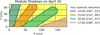 |
Fig. 6 Module shadows at several hours on April 16. |
 |
Fig. 7 Module shading patterns with centroid-based intersection at 1 × 1 cell resolution. |
 |
Fig. 8 Module shading patterns with centroid-based intersection at 2 × 2 sub-cell resolution. |
 |
Fig. 9 Distributions of cell shading fractions across all 40 cells and 4 solar positions (April 16, 14:00, 15:00, 16:00, 17:00), evaluated with centroid-based approach at resolutions from 1 × 1 to 4 × 4. |
3.1.1 Shadow validation
The accuracy of the vertex projection method is demonstrated in Figures 10–12, where the simulated shadow positions are compared with the captured images at different times of the day, and they match very closely. In Figure 10, we compare the simulation result with the observed shadow at the moment when the shadow begins to appear on the module, at 13:23 local time on April 16. At this moment, captured in Figure 10b, the shadow appears as just a small sliver running along the left edge of the module. The module area is highlighted by the blue rectangle, in order to avoid confusion, since the top row of tiles are ordinary roof tiles and not part of the PV module. In the simulation on the left, the red line indicates the contour of the shadow, the black lines indicate the tiles, and the dark grey lines represent the regions containing each cell. In the image on the right, the cells themselves are not visible, but they are arranged in tiles, which are visible in two sizes. The wider tiles each consist of a row of 4 cells, and the smaller tiles are made of a row of 2 cells.
Next, Figure 11 shows the results at 15:06 local time, and this time was chosen for validation because the shadow spans just to the top of the module. We see that the position of the shadow on all tiles is correct.
Figure 12 shows the position of the shadow at 16:49, the last recorded time when the shadow was still visible on the bottom of the module, before dense clouds arrived. We see that on the right edge, the shadow spans to the top of the second row of tiles from bottom.
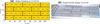 |
Fig. 10 (a) Simulated shadow compared to (b) observed shadow at 13:23:50. |
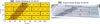 |
Fig. 11 (a) Simulated shadow compared to (b) observed shadow at 15:06:04. |
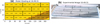 |
Fig. 12 (a) Simulated shadow compared to (b) observed shadow at 16:49:31. |
3.1.2 Cell shadings analysis
Figure 13 presents the evolution of the maximum shaded fraction over the afternoon period when shading occurs on April 16. Results for obstacle diameters of 5 cm, 10 cm, and 25 cm are shown in Figures 13a–13c, with the 25 cm case corresponding to the experimental setup. The shaded fraction at each time is the maximum value across all cells or sub-modules. Varying the point sampling approach, we show the cell centroid model at several resolutions, the sub-module corner model, and the conservative baseline, which assumes full shading if any point on the module is shaded.
In the 25 cm scenario, the shadow width is comparable to the cell diagonal, so at any given time as the shadow passes over the module, at least one cell is fully or nearly fully shaded. As a result, the maximum shaded fraction across all cells remains at or very close to 1 for most of the afternoon. Like the conservative baseline on this day, the sub-module model calculates that the shaded fraction jumps from 0 to 1 at 13:18, as soon as the shadow touches the edge of the module (a few minutes before the photo in Fig. 10). The shaded fraction remains 1 until the shadow completely disappears at 17:33. At 1 × 1 resolution, the cell centroid model predicts a jump from 0 to 1 at 13:33, when the shadow reaches halfway across the top left cell and intersects its centroid. It then predicts full shading until 17:27, when the shadow is halfway across the bottom right cell and no longer intersects its centroid.
Cell partial shading is captured by the cell centroid model beginning at a resolution of 2 × 2. This becomes evident during the shadow transitions onto and off of the module, when the most shaded cell is only partially shaded over 24 min periods in the early and late afternoon. At 40 × 40 resolution, the model also detects a slight mid-afternoon oscillation, which arises from the alignment between the shadow and the cells. As seen in Figure 11, where the shadow lies at a nearly 45° angle across the module, the most shaded cell can still be partially shaded when a shadow of this size crosses the module diagonally.
When the obstacle diameter is reduced to 5 cm or 10 cm, the shadows produced are narrower than a cell, leading to cell partial shading over the entire shading period. With the cell centroid model, the violet curves at 40 × 40 resolution show that the shaded fraction of the most shaded cell follows a relatively smooth profile over the course of the day. Lower resolutions of 2 × 2 and 3 × 3, shown in yellow and green, produce visible oscillations but already begin to approximate this profile.
However, the issue of missed shadow detections becomes visible in the thinner obstacle scenarios, as the shaded fraction sometimes falls to 0 even while the shadow is still on the module. These events occur with both the sub-module model and the cell-level model at 1 × 1 resolution, because the points tested for shadow intersection are spaced farther apart than the shadow width, allowing some shadings to pass undetected. As expected, the narrower 5 cm shadow is missed more frequently than the 10 cm one.
The sub-module model departs from the conservative baseline only during these missed shadow events. In the module examined in this study, the sub-modules contain only two or four cells and alternate in arrangement, so their corners are relatively close. With larger sub-modules, non-alternating layouts, or thinner shadows, the likelihood of missed detections would increase.
The cell centroid model samples points more densely, but at 1 × 1 resolution it can still miss 5 cm and 10 cm shadows. As the cell region is roughly 17.5 cm wide, a 2 × 2 resolution samples points less than 9 cm apart, which is sufficient to detect the 10 cm shadow. It also captures the 5 cm shadow on this particular day, although sampling points less than 5 cm apart for year-round detection requires a 4 × 4 resolution. In general, the spacing between sampled points should be small enough to reliably detect shadows. Once this condition is met, the cell-level model at 2 × 2 resolution or higher can be used to estimate cell partial shading.
Because the resolution is defined relative to the cell size, we also expect higher resolutions to be more relevant for larger cells, where partial cell shading is more likely. In the case of half cells, rectangular resolutions such as 2 × 4, rather than square resolutions like 2 × 2, should achieve a more uniform sampling of points over the cell surface. Therefore, selecting shadow intersection sampling points based on the shadow and cell sizes is an interesting direction to further explore with a cell level approach.
In Figure 14, we show the mean shaded fraction across all hours of the year, comparing the cell centroid and cell corner models at different resolutions, as well as the sub-module corners model, against the conservative baseline. The difference between the sub-module model and the conservative baseline corresponds to missed shadow detections. As expected, thinner shadows produce more such events and thus a larger difference.
The cell centroid model and the cell corners model converge at very high resolution to the same mean annual shaded fraction, about 18.3% for the 25 cm obstacle, but the centroid model converges faster. This is expected because the corner-based logic is conservative, whereas centroid-based logic is on average more balanced. In the 25 cm scenario, the mean shaded fraction predicted by the cell centroid model is already within 0.4% of the convergence value at a resolution of 1 × 1 (1 in the figure). At this resolution, the model does not explicitly account for partial cell shading because the shaded fraction at any time is either 0 or 1. Even so, it provides a close estimate of the mean shaded fraction because partial shading occurs mainly during the shadow transition periods, which are balanced on average by the centroid-based detection logic.
In the 10 cm case, the cell centroid and cell corner models converge at resolutions well above 40 × 40, but between 10 × 10 and 40 × 40 the cell centroid model already stabilizes at a mean shaded fraction of 11.4%. Using the cell centroid model at a resolution of 2 × 2 avoids missed shadings and begins to account for cell partial shading throughout the afternoon, estimating the mean shaded fraction within 1.6% of the 40 × 40 value. The difference decreases to 0.6% at 3 × 3 resolution and 0.3% at 4 × 4 resolution as partial shading is estimated more precisely.
The cell models converge at even higher resolution in the 5 cm case, but again the cell centroid model stabilizes between 10 × 10 and 40 × 40 resolution, at a mean shaded fraction of 6.1%. The estimate at 4 × 4 resolution is already within 0.4% of the 40 × 40 value.
Therefore, the mean shaded fraction predicted by the cell centroid model stabilizes at higher resolutions for the thinner 10 cm and 5 cm shadows. Still, even in these cases, it can be estimated within 0.4% of the 40 × 40 value at a resolution of only 4 × 4, showing little benefit by going to higher resolutions. At 40 × 40 resolution, the model predicts lower mean shaded fractions for the thinner shadows because they produce less partial shading on the cells. The difference between these 40 × 40 values and the conservative baseline mean indicates the impact of partial cell shading. As expected, the cell centroid model captures partial cell shading in all three scenarios, with thinner shadows producing a lesser extent of partial shading and therefore a larger deviation from the baseline.
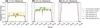 |
Fig. 13 Shaded fractions modeled at 3 min intervals on April 16 for obstacle diameters of (a) 5 cm, (b) 10 cm, and (c) 25 cm. The shaded fraction at each time is that of the most shaded cell or sub-module. Results from the cell centroid model at resolutions of 1 × 1, 2 × 2, 3 × 3, and 40 × 40 are compared to the conservative baseline and the sub-module corner model. |
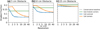 |
Fig. 14 Annual average of hourly maximum shading fractions for 5 cm, 10 cm, and 25 cm obstacles. The means computed at multiple resolutions using the cell centroid and cell corner models and the sub‑module corners model are compared to the conservative baseline. |
3.2 Irradiance analysis
The ground irradiance measurements from April 13 are presented in Figure 15. Because April 16 was an overcast day, with shading occurring at only a few moments when the sun came out of the clouds, we instead chose April 13, a sunny day, to compare the shading models.
In Figure 16, we present the relative irradiance loss on April 13, comparing the sub-module and cell centroid models to the conservative baseline for the three obstacle sizes. The irradiance loss is directly proportional to the shaded fraction ((Eq. 8)), but unlike the latter, it is also dependent on the weather. On this sunny day, the relative irradiance loss profile resembles that of the shaded fraction, but the irradiance losses become smaller in the late afternoon, after 16:30, when the sky becomes slightly overcast.
During the early and late afternoon shadow transition periods, partial cell shading occurs with all three obstacle sizes. Like the conservative baseline, the sub-module model predicts higher irradiance losses over these periods than the cell centroid model.
During the mid-afternoon period, in the 25 cm case, the most shaded cell remains fully or nearly fully shaded. Thus, the maximum irradiance loss remains at or very close to the conservative baseline. The sub-module model aligns with the conservative baseline, as the favorable sub-module geometry helps it avoid missed detections on this day. At 40 × 40 resolution, the cell centroid model captures small deviations from the conservative baseline due cell partial shading when the 25 cm shadow crosses the module diagonally. Otherwise, these deviations are too small to be captured at the lower resolutions.
In the 10 cm and 5 cm scenarios, the most shaded cell remains partially shaded throughout the afternoon. The sub-module model deviates from the conservative baseline only at times when it predicts no irradiance loss due to a missed shadow. Starting at 2 × 2 resolution, the cell centroid model predicts lower irradiance losses than the conservative baseline, as it captures the cell partial shading.
Figure 17 presents the annual mean relative irradiance loss over hourly TMY data, for obstacle diameters of 5 cm, 10 cm, and 25 cm. In the 25 cm case, the sub-module model predicts a mean only 0.02% lower than the conservative baseline. Because the shadow is narrower than the sub-modules, it is susceptible to miss shadings, which may occur more or less frequently depending on the size and arrangement of the sub-modules relative to the shadow. The relatively small size of the sub-modules and their favorable alternating arrangement in the module causes these events to be rare for the 25 cm shadow. Yet as the shadow becomes thinner, they naturally become more frequent, lowering the mean predicted by the sub-module model relative to the conservative baseline. The difference of 2.8% in the 10 cm case, and 8.6% in the 5 cm case can be attributed entirely to missed shadow detections.
Comparing the cell centroid model at 40 × 40 resolution against the conservative baseline, we estimate the losses potentially recovered by accounting for partial cell shading. For the 25 cm shadow, the difference of 1.96% mainly results from sunny shadow transition periods in the early and late afternoon. Due to the hourly time resolution of the TMY data, only a fraction of these are captured, but they are enough to make a noticeable difference in the annual mean. We note that the annual mean may still be influenced by the hourly temporal resolution. For the 10 cm and 5 cm shadows, the differences of 10.5% and 17.6% arise from cell partial shading throughout the afternoon mainly because the shadows are narrower than the cell.
In this analysis, we evaluated the irradiance losses predicted by the different strategies to check points for shadow intersection. Because the cells are connected in series, we conservatively assume the module current is limited by the most shaded cell, and the irradiance loss is therefore defined using the minimum cell irradiance at each time step. This choice provides a consistent basis for comparing point sampling strategies but also introduces several important considerations.
This worst-case definition does not incorporate the effects of bypass diode activation or the module’s operating point on the I-V curve. As such, the irradiance losses reported here should be interpreted as upper bounds on shading impact at the cell level. Within this conservative framework, the difference between the baseline and the modeled results reflects the relative influence of partial cell shading rather than an estimate of recoverable DC energy.
A second limitation is that the analysis remains fully model based. The diffuse plane-of-array irradiance is derived from measured DHI and GHI rather than directly measured, and no comparison was performed against measured module or string performance under partial shading. As a result, the quantitative values presented here represent model predictions rather than experimentally validated metrics.
Despite these limitations, the results suggest that modeling partial shading on individual cells can meaningfully alter predicted near shading losses, particularly for thin shadows. In any case, these findings should be corroborated on data from a wider variety of shadow configurations and cell sizes.
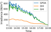 |
Fig. 15 Measured 3 min GPOA, DHI, and GHI irradiance data on the afternoon of April 13. |
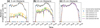 |
Fig. 16 Maximum relative irradiance loss over the cells or sub-modules, modeled using 3 min irradiance measurements on April 13, for 5 cm, 10 cm, and 25 cm obstacles. The cell centroid model at several resolutions and the sub-module model are compared to the conservative baseline. |
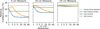 |
Fig. 17 Annual mean relative irradiance losses computed for 5 cm, 10 cm, and 25 cm obstacles, using the cell-level corner and centroid models at varying resolutions, compared to the submodule-level model and conservative baseline. |
3.3 Runtime analysis
In Figure 18, we explore the impact of the resolution and number of cells on the 1-yr hourly calculation time using the 2D method. Figure 18a shows how increasing the resolution in the 40-cell configuration affects the simulation time of the models. The cell centroid model requires around 17 s at resolutions up to 5 × 5. Because the number of sample points increases with the square of the resolution, we might expect the runtime to grow rapidly. In practice, the increase is modest at resolutions below 10 × 10 because the sample point calculation is vectorized and therefore handled efficiently. Only at higher resolutions does the quadratic growth become evident.
A consistent trend across all resolutions is that the cell corner model runs slightly slower than the cell centroid model. This is expected, as each sub-cell contributes four corner points instead of a single centroid, increasing the number of sample points. At low resolutions the difference is small, but it grows with resolution and becomes very large at high resolutions. Also, the sub-module model is a few seconds faster than the 1 × 1 cell centroid model because it avoids the interpolation step to generate sample points.
In Figure 18b, we vary the number of cells in the model configuration to observe how it affects the runtime, using the cell centroid model at various resolutions. The figure shows that runtime is more or less linearly dependent on the number of cells, and the slope increases with resolution. For resolutions of 3 × 3 and below, the runtime grows relatively slowly with the number of cells, remaining between 19 and 24 s for a simulation with 1200 cells.
For comparison, a linear shadings simulation was also done in PVsyst 7.4.7, using both the fast shadings calculation that interpolates shading factors from a precomputed table, and the slow simulation that evaluates the shading factor at every solar position. The slow mode in PVsyst remains a few seconds faster than our sub-module simulation, suggesting there is still room to optimize the implementation. Potential improvements include reducing the number of intermediate data structures and using more efficient numerical operations.
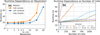 |
Fig. 18 Runtime of the simulation on hourly TMY data: (a) at varying resolution, comparing different models in the 40-cell configuration, and (b) increasing the number of cells, using the cell centroid model at various resolutions. |
3.4 Future work
The cell-level near shading approach presented in this study offers an improvement in spatial resolution over a conventional submodule-level approach, suggesting that it could enable more accurate irradiance estimates under partial shading conditions. By computing the plane-of-array irradiance on each cell adjusted for shading, the model provides a means for evaluating irradiance losses and supports future integration with electrical simulations. While this work focuses on modeling partial cell shading and quantifying irradiance losses, it does not go so far as to compute electrical losses. Therefore, future work will aim to extend this framework by integrating the irradiance model with temperature and electrical modeling to determine energy yield losses. In this work, the shading model was built and validated on an experimental configuration, and future work will explore a variety of model configurations across different shadow and cell sizes. Validation is also needed to confirm the accuracy of the modeled shading-adjusted irradiance and to translate it into reliable energy yield estimates.
At the same time, the current approach to resolve the shaded fraction per cell, based on binary shadow intersection logic, is suited to configurations where irradiance is homogeneous over the shaded regions. However, it does not represent spatial variations within the shaded area of a cell, which may limit its ability to capture inhomogeneous shadings such as penumbra or soft shadows, especially those caused by narrow obstructions like rods, cables, or wires [9]. In such scenarios, we expect that computing irradiance via ray tracing would be more appropriate, and this represents a logical extension for future work. Additionally, while ray tracing is computationally expensive, GPU acceleration could reduce the ray tracing simulation time and help with developing a cell-level near shading model better suited to very thin obstructions.
4 Conclusion
This study introduces a near shading model for photovoltaic modules at the cell level. Starting with ground irradiance data, we simulate the shadow position using vertex projection, compute the cell shading fractions, and finally the cell shading-adjusted plane-of-array irradiance. A 2D vertex projection shadow modeling approach was developed, and we validated the shadow positions experimentally. We began to explore the potential to improve the accuracy of cell shading fractions and irradiance losses by choosing to check more points for shadow intersection, observing that compared to the conservative full-shading baseline model, the cell-level model accounting for cell partial shading may predict a 1.96% lower mean annual irradiance loss for a 25 cm wide shadow and even more for thinner shadows. This difference, however, should be interpreted as an upper bound to recoverable power losses with a cell-level model, not accounting for bypass diode mitigation or I-V behavior. At sufficient resolution, the cell-level approach avoids missing shadow detections observed with the sub-module approach. The tradeoff is on computation time, which increases with the resolution and the number of cells. The 1-yr hourly simulation using the cell centroid model with a resolution between 2 × 2 and 5 × 5 points per cell runs in around 17 s, and the sub-module model in about 13 s, which is still several seconds slower than PVsyst. While we believe the implementation could be further optimized, we observed that this algorithm scales efficiently with the number of cells at lower resolutions, running in about 25 s at a 3 × 3 resolution for 1200 cells. Future work will further investigate the impact of shadow and cell sizes on optimal resolution. These findings encourage future work to increase the accuracy of irradiance modeling at the cell level, especially for applications where smaller shadows are often present such as BIPV. The method developed in this work provides a base for future integration with thermal and electrical modeling, which could be used to calculate the energy yield, and further experimental validation will be important to ensure the modeled shading-adjusted irradiance translates into reliable energy yield estimates. This work could therefore be of interest when simulating performance of smaller PV systems exposed to thinner shadows.
Acknowledgments
The authors would like to thank Cédric Bucher and Nicolas Furst for building the chimney structure used in the experiment, and Florian Ollagnon for the STC IV measurements of the solar tiles.
Funding
This research was funded by the European Union’s Horizon Europe, Innovation Actions programme under grant agreement No. 101136112 (Increase Project), No. 101136094 (Sphinx Project), and No. 101172767 (Empower project). This work has received funding from the Swiss State Secretariat of Education, Research and Innovation (SERI).
Conflicts of interest
The authors have nothing to disclose.
Data availability statement
The data supporting the findings of this study are available upon reasonable request. Due to resource limitations, the data are not hosted in a public repository.
Author contribution statement
Conceptualization, J.-P.C. and A.F.; Methodology, J.-P.C.; Software, J.-P.C., F.M., and J.L.; Validation, J.-P.C. and A.F.; Formal Analysis, J.-P.C.; Investigation, J.-P.C.; Resources, J.-P.C., P.R., K.N.; Data Curation, J.-P.C.; Writing – Original Draft Preparation, J.-P.C.; Writing – Review & Editing, All authors; Visualization, J.-P.C.; Supervision, A.F.; Project Administration, J.-P.C. and A.F.; Funding Acquisition, A.F.
References
- A. Mermoud, PVSYST: a user-friendly software for PV-systems simulation, in Twelfth European Photovoltaic Solar Energy Conference: proceedings of the International Conference (1994) [Google Scholar]
- B.A. de Sá, T. Dezuo, D. Ohf, Shadow modelling algorithm for photovoltaic systems: extended analysis and simulation, J. Control Autom. Electr. Syst. 33, 1507 (2022). https://doi.org/10.1007/s40313-022-00905-2 [Google Scholar]
- M.A. Mikofski, M. Lynn, J. Byrne, M. Hamer, A. Neubert, J. Newmiller, Accurate performance predictions of large PV systems with shading using submodule mismatch calculation, in 2018 IEEE 7th World Conference on Photovoltaic Energy Conversion (WCPEC) (A Joint Conference of 45th IEEE PVSC, 28th PVSEC & 34th EU PVSEC) (Jun. 2018), pp. 3635–3639. https://doi.org/10.1109/PVSC.2018.8547323 [Google Scholar]
- B. Meyers, M. Mikofski, M. Anderson, A fast parameterized model for predicting PV system performance under partial shade conditions, in 2016 IEEE 43rd Photovoltaic Specialists Conference (PVSC) (Jun. 2016), pp. 3173–3178. https://doi.org/10.1109/PVSC.2016.7750251 [Google Scholar]
- K.S. Anderson, C.W. Hansen, W.F. Holmgren, A.R. Jensen, M.A. Mikofski, A. Driesse, pvlib python: 2023 project update, J. Open Source Softw. 8, 5994 (2023). https://doi.org/10.21105/joss.05994 [CrossRef] [Google Scholar]
- P.G. Loutzenhiser, H. Manz, C. Felsmann, P.A. Strachan, T. Frank, G.M. Maxwell, Empirical validation of models to compute solar irradiance on inclined surfaces for building energy simulation, Sol. Energy 81, 254 (2007). https://doi.org/10.1016/j.solener.2006.03.009 [Google Scholar]
- H.C. Hottel, B.B. Woertz, The performance of flat-plate solar-heat collectors, Trans. Am. Soc. Mech. Eng. 64, 91 (2022). https://doi.org/10.1115/1.4018980 [Google Scholar]
- A. Martinez, PVGIS photovoltaic geographical information system, JRC Publications Repository. Accessed: Sep. 16, 2024. [Online]. Available: https://publications.jrc.ec.europa.eu/repository/handle/JRC142887 [Google Scholar]
- M. Axisa, M. Demicoli, L. Mule’Stagno, Analysing the effects of thin object shading on PV sources: a dual approach combining outdoor and laboratory solar simulator experimentation, Energies 17, 2069 (2024). https://doi.org/10.3390/en17092069 [CrossRef] [Google Scholar]
Cite this article as: Jean-Paul Calin, Jacques Levrat, Antonin Faes, Fahradin Mujovi, Paul Rémondeau, Kléber Nicolet-dit-Félix, Bénédicte Bonnet-Eymard, Didier Dalmazzone, Aïcha Hessler-Wyser, Christophe Ballif, Modeling partial shading at the cell level on photovoltaic modules, EPJ Photovoltaics 17, 23 (2026), https://doi.org/10.1051/epjpv/2026015
All Figures
|
Fig. 1 3D Vertex projection approach: (a) model configuration, (b) vertices projected on ground plane, (c) 3D shaded region, (d) cell shadow raster, (e) module shadow. |
| In the text | |
|
Fig. 2 2D approach: (a) model configuration, (b) obstacle vertices projected onto ground plane, (c) 2D shadow polygon, (d) cell corners projected onto ground plane, (e) points sampled at desired resolution on ground plane, (f) point-in-polygon test for shadow intersection. |
| In the text | |
|
Fig. 3 Runtime per solar position of the 3D and 2D methods at different resolutions. |
| In the text | |
|
Fig. 4 Comparison of methods to determine which points to check for shadow intersection. Corner-based (top) vs. centroid-based (bottom) intersection logic. Point sampling at submodule-level (left) vs. cell-level at resolution 1 × 1 (center) and 2 × 2 (right). |
| In the text | |
|
Fig. 5 Experimental setup for partial shading on BIPV roof tiles: (a) front view, (b) side view. |
| In the text | |
|
Fig. 6 Module shadows at several hours on April 16. |
| In the text | |
|
Fig. 7 Module shading patterns with centroid-based intersection at 1 × 1 cell resolution. |
| In the text | |
|
Fig. 8 Module shading patterns with centroid-based intersection at 2 × 2 sub-cell resolution. |
| In the text | |
|
Fig. 9 Distributions of cell shading fractions across all 40 cells and 4 solar positions (April 16, 14:00, 15:00, 16:00, 17:00), evaluated with centroid-based approach at resolutions from 1 × 1 to 4 × 4. |
| In the text | |
|
Fig. 10 (a) Simulated shadow compared to (b) observed shadow at 13:23:50. |
| In the text | |
|
Fig. 11 (a) Simulated shadow compared to (b) observed shadow at 15:06:04. |
| In the text | |
|
Fig. 12 (a) Simulated shadow compared to (b) observed shadow at 16:49:31. |
| In the text | |
|
Fig. 13 Shaded fractions modeled at 3 min intervals on April 16 for obstacle diameters of (a) 5 cm, (b) 10 cm, and (c) 25 cm. The shaded fraction at each time is that of the most shaded cell or sub-module. Results from the cell centroid model at resolutions of 1 × 1, 2 × 2, 3 × 3, and 40 × 40 are compared to the conservative baseline and the sub-module corner model. |
| In the text | |
|
Fig. 14 Annual average of hourly maximum shading fractions for 5 cm, 10 cm, and 25 cm obstacles. The means computed at multiple resolutions using the cell centroid and cell corner models and the sub‑module corners model are compared to the conservative baseline. |
| In the text | |
|
Fig. 15 Measured 3 min GPOA, DHI, and GHI irradiance data on the afternoon of April 13. |
| In the text | |
|
Fig. 16 Maximum relative irradiance loss over the cells or sub-modules, modeled using 3 min irradiance measurements on April 13, for 5 cm, 10 cm, and 25 cm obstacles. The cell centroid model at several resolutions and the sub-module model are compared to the conservative baseline. |
| In the text | |
|
Fig. 17 Annual mean relative irradiance losses computed for 5 cm, 10 cm, and 25 cm obstacles, using the cell-level corner and centroid models at varying resolutions, compared to the submodule-level model and conservative baseline. |
| In the text | |
|
Fig. 18 Runtime of the simulation on hourly TMY data: (a) at varying resolution, comparing different models in the 40-cell configuration, and (b) increasing the number of cells, using the cell centroid model at various resolutions. |
| In the text | |
Current usage metrics show cumulative count of Article Views (full-text article views including HTML views, PDF and ePub downloads, according to the available data) and Abstracts Views on Vision4Press platform.
Data correspond to usage on the plateform after 2015. The current usage metrics is available 48-96 hours after online publication and is updated daily on week days.
Initial download of the metrics may take a while.