© A. Bourgeois et al., Published by EDP Sciences, 2026

1 Introduction

Due to the rapid development of perovskite-based tandem solar cells, tandem devices are projected to capture a significant part of the solar cell market in the next decade [1,2]. With this momentum comes an increasing demand for accurate and accessible characterization to support transparent reporting of tandem devices in both academia and industry. Among all characterization metrics, the current–voltage (I–V) measurement under Standard Testing Conditions (STC) remains the most critical, as it determines the efficiency and maximum power output of the device.

The I–V measurements of tandem solar cells are highly sensitive to the spectral characteristics of the incident illumination. In a laboratory setting, the discrepancy between the reference spectrum and the simulated spectrum generated by a solar simulator can substantially distort I–V measurements, affecting both short-circuit current and fill factor. To avoid these distortions, the solar cell’s behavior under the simulated spectrum must mirror its behavior under the reference spectrum [3].

This condition was formalized in the standard IEC 60904-1-1: Measurement of current-voltage characteristics of multi-junction photovoltaic devices. The IEC defines two metrics, mismatch factor M and matching factor Z.

$$M=\frac{{\displaystyle {\int }_{}^{}}{E}_{\text{sim}}(\lambda ){\text{SR}}_{\text{DUT}}(\lambda )d\lambda {\displaystyle {\int }_{}^{}}{E}_{\text{ref}}(\lambda ){\text{SR}}_{\text{RC}}(\lambda )d\lambda }{{\displaystyle {\int }_{}^{}}{E}_{\text{ref}}(\lambda ){\text{SR}}_{\text{DUT}}(\lambda )d\lambda {\displaystyle {\int }_{}^{}}{E}_{\text{sim}}(\lambda ){\text{SR}}_{\text{RC}}(\lambda )d\lambda }$$(1)

$$Z=\frac{I_{\text{RC}}^{\text{ref}}}{I_{\text{RC}}^{\text{sim}}M}$$(2)

where E_ref is the reference spectrum (typically Air Mass 1.5 Global, or AM1.5G for short), SR_RC, SR_DUT are the spectral responses of the reference solar cell(s) and the Device-Under-Test respectively, E_sim is the spectrum of the solar simulator, $I_{\text{RC}}^{\text{ref}}$ is the reference solar cell’s current under the reference spectrum, and $I_{\text{RC}}^{\text{sim}}$ is the measured reference solar cell current under the solar simulator.

IEC 60904-1-1 stipulates that a calibrated spectrum for measurement of a tandem solar cell must meet the following criteria:

• M_top, M_bot, must satisfy M_top, M_bot = 1.00±0.05 to be considered spectrally approximated.

• Z_top, Z_bot, must achieve Z_top, Z_bot = 1.00±0.03, and target 1±0.01.

Two additional conditions concerning the current-limiting junction and current balance are also desirable, but their examination falls outside the scope of this work [4].

While the standard defines the target criteria without prescribing a specific methodology, the literature contains several methods to achieve them. Specifically for multi-LED (Light Emitting Diode) solar simulators – which offers considerable ease of spectral tuning – several studies have shared the calibration procedures for multi-junction solar cells [5,6]. These studies are important resources for those aiming to achieve a high level of calibration accuracy. Nevertheless, the methods presented may be difficult to reproduce for those who need a readily available calibration. This study shares a calibration method with open-source code that target the requirements of IEC 60904-1-1.

This study is structured as follows: Section 2.1 describes the materials used. Section 2.2 details the prerequisite capabilities of the solar simulator required for the calibration and outlines methods to enable them if not readily available. The calibration methodology is presented in Section 2.3, followed by the results in Section 3. A discussion of the method’s strengths and limitations is provided in Section 4. The corresponding code implementation is available at: https://github.com/Stella-Hdw/Multi-LED-Solar-Simulator-Calibration-for-Tandem-I-V.

2 Materials and method

2.1 Materials

A WAVELABS Sinus-220 solar simulator, comprising 21 LEDs, was used in this study. The spectral irradiance of each LED at maximum power is shown in Figure 1. The reference solar cells (RC) used for the calibration were World PV Scale Standard (WPVS) reference solar cells: a KG3-filtered silicon solar cell for the top reference sub-cell and a BL7-filtered silicon solar cell for the bottom reference sub-cell. Their external quantum efficiency (EQE) is shown in Figure 2 in grey. Their spectral response and short-circuit current under the reference spectrum were certified by the vendor [7].

Spectral irradiance was measured using a Raysphere 1700 spectrometer (Ocean Optics). The instrument’s visible and near-infrared detectors are calibrated annually by the manufacturer, with the spectral irradiance standard used for calibration being traceable to SI units via National Institute of Standards and Technology (NIST)-certified reference lamps.

All measurements were conducted with the reference solar cells mounted on a temperature-controlled stage maintained at 25 °C. The reference solar cells’ temperature were assumed to remain stable at 25 °C during the brief flash measurements. The devices under test were 1 cm² perovskite-silicon tandem solar cells. Their EQE was characterized using an Enlitech QE-R system, with the spectral response of the Si and Ge detectors calibrated by the manufacturer and traceable to NIST standards.

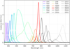Fig. 1 Spectral irradiance of the LEDs at maximum power of the solar simulator used.

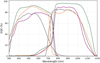Fig. 2 EQE of reference solar cells (grey), and tandem solar cells (A in orange, B in purple, C in green).

2.2 Solar Simulator

The solar simulator generates a composite spectral irradiance, E_sim, from m individual LEDs. Each LED j is controlled by a parameter α_j ∊ [0,1], where α_j = 0 corresponds to the LED being off and α_j = 1 to its maximum output. The complete set of control parameters is denoted by {α} = {α₁, α₂,...,α_m}. The calibration method presented herein requires the user of the solar simulator to possess the following three capabilities:

• Independent Control and Spectral Measurement: The user can set each control parameter α_j independently and measure the resulting spectral irradiance with a spectrometer.

• Spectral Calculation: The total spectral irradiance E_sim can be calculated for any given set {α}.

• Spectrum Fitting: The simulator can generate a spectrum E_sim that approximates a target reference spectrum E_ref, and the corresponding set {α} that produced this spectrum is known.

These are henceforth referred to as Capabilities 1, 2, and 3. As some solar simulators may not provide Capabilities 2 and 3 directly, the following subsections describe how to enable them using the fundamental Capability 1.

2.2.1 Capability 2: Calculating the spectrum from control parameters

The total spectral irradiance is defined as the sum of the spectral irradiances from all individual LEDs¹:

$$E_{\text{sim}}(\lambda )={\displaystyle \sum _{j=1}^m}{E}_j(\lambda \mathrm{,}{\alpha }_j)\mathrm{}$$(3)

An ideal, linear model would define the spectral irradiance of LED j as $E_j({\mathrm{\lambda ,\alpha }}_j)={\alpha }_j{e}_j(\lambda )$, where e_j(λ) is the spectrum at maximum power (α_j = 1). However, thermal effects, notably spectral red-shifting, cause significant deviation from this linear relationship [5,8,9]. To account for this non-linearity, each LED j is characterized empirically by measuring its spectrum at discrete control values ${\alpha }_j\in \left\{\mathrm{0.1,0.2,...,1.0}\right\}$. Although the LED is globally nonlinear, we assume approximate local linearity between 10% intervals (see Appendix, Fig. A1). For a given α_j, the spectrum E_j(λ,α_j) is constructed via linear interpolation between the two nearest pre-characterized values [5,8].

2.2.2 Capability 3: Spectrum Fitting

We developed a basic spectrum-fitting algorithm by implementing Nelder-Mead optimization with α constrained to [0,1], to act as the ‘base’ spectrum. Nelder-Mead optimization is a commonly-used numerical, heuristic, and direct method for finding local minima of an objective function [10].

The base spectrum only optimizes for spectral shape (minimizing its difference with AM1.5G) and not the spectral response of the device under test. The base spectrum is henceforth used for comparison with ’calibrated’ spectra which take into account the tandem sub-cell responses according to IEC 60904-1-1.

2.3 Calibration

The visualization of some steps in the calibration method explained in this section can be found in Figure 4. The calibration process is initiated by generating a base spectrum, $E_{\text{sim}}^{\text{base}}$, through Capability 3, yielding the corresponding control parameters {α^base}.

The system of equations to solve, presented in Meusel’s method (see Appendix) is under-determined, as a tandem solar cell provides only two equations for the m > 2 control parameters of a multi-LED solar simulator (Meusel et al. [11]). To constrain the problem, the m LEDs are partitioned into two virtual light sources, E_I and E_II, by defining a split point k. The first k LEDs, sorted by increasing peak wavelength, form E_I, while the remaining m – k LEDs form E_II (Fig. 4A, solid lines). Application of Meusel’s method yields calibrated intensity factors A_I and A_II for the virtual lamps. The corresponding calibrated control parameters for a given split k are then computed as:

$${\alpha }_j^{\text{Meusel}\mathrm{,}k}=\{\begin{array}{cc}{A}_{\text{I}}{\alpha }_j^{\text{base}},& \text{for}\hspace{1em}j\le k\\ A_{\text{II}}{\alpha }_j^{\text{base}}\mathrm{,}& \text{for}\hspace{1em}j>k\end{array}$$(4)

The virtual spectrum E^Meusel,k is calculated (Fig. 4). This procedure is iterated over all possible split points k ∊ [1, m–1]. Each spectrum’s mismatch factor is also calculated. The optimal virtual spectrum, $E_{\text{sim}}^{\text{Meusel}\mathrm{,}k=\text{best}}$, is selected by minimizing the deviation of the average mismatch factor from unity (Fig. 4B). When multiple splits yield comparable performance of the mismatch factor, the spectral match classification per IEC 60904-9 can serve as a secondary selection criterion [12]. The concept of grouping the LEDs into the number of junctions is also discussed in [6]. However, in [6], instead of being empirically chosen by the mismatch factor, k is decided by the band-gaps of the sub-cells. The implication of this decision is discussed in Section 3.2.

The generation of $E_{\text{sim}}^{\text{Meusel}\mathrm{,}k=\text{best}}$ requires translation of the idealized coefficients $\left\{{\alpha }_j^{\text{Meusel}\mathrm{,}k=\text{best}}\right\}$ into physically realizable control parameters. These coefficients assume a linear relationship between input and spectral output, inherent in the linear system of equations formulated by Meusel’s method. This assumption is invalidated by LED non-linearity (Sect. 2.2.1). Two methods can be used to determine the true control parameters {α^calib}: (1) application of a polynomial correction to account for non-linear response (explained in the Appendix, used in this study) [5], or (2) direct spectrum fitting to target $E_{\text{sim}}^{\text{Meusel}\mathrm{,}k=\text{best}}$ using Capability 3. An example of the change from {α^base} to {α^calib} is shown in Figure 4C.

To ensure the physically realized spectrum $E_{\text{sim}}^{\text{calib}}$ is the same as the simulated spectrum $E_{\text{sim}}^{\text{Meusel}\mathrm{,}k=\text{best}}$, $E_{\text{sim}}^{\text{calib}}$ is measured using a spectrometer. The simulated and measured spectra and compared. The measured spectra enables recalculation of M_top and M_bot with the true spectrum as opposed to the virtual $E_{\text{sim}}^{\text{Meusel}\mathrm{,}k=\text{best}}$. If a repeatable similarity between simulated and measured spectra is established, one can practically assume that the two spectra are equivalent with a given uncertainty, and thus forgo the need to measure the spectrum again to recalculate M_top and M_bot for Z, accelerating the calibration process. Nevertheless, measuring the calibrated spectrum gives the most confidence on the M_top and M_bot values and is recommended.

Once M_top and M_bot are known, subsequent measurement of reference solar cell short-circuit currents ($I_{\text{top,RC}}^{\text{sim}}$ and $I_{\text{bot,RC}}^{\text{sim}}$) under this calibrated spectrum allows computation of the final matching factors Z_top and Z_bot. The calibration is considered satisfactory if both Z-factors satisfy the criterion |1–Z|≤0.03.

3 Results

3.1 Z and M after calibration

The calibration method was tested on three perovskite-silicon tandem solar cells, referred to as Cell A, B and C. The EQE of the reference solar cells and the tandem solar cells, used to calculate the spectral response, are shown in Figure 2. The measured calibrated spectra of each cell is shown in Figure 3, along with the base spectrum. The mismatch factor and matching factor of the base and calibrated spectra are shown in Table 1. For the mismatch factor, almost all cells had |1–M|>0.05 for the base spectrum. After calibration, the calibrated spectra are ‘approximately spectrally matched’, achieving |1–M|<0.05. For the matching factor, the base spectrum, which was fitted only with approaching the AM1.5G spectral shape as an objective, did not meet the criteria, with most |1–Z|>0.03 (with the exception of Cell B, bottom). After calibration, |1–Z|<0.03 for all matching factors. Thus, the IEC 60904-1-1 requirements are fulfilled after calibration.

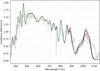Fig. 3 Reference spectrum (AM1.5G) (in grey), base spectrum (in black) and calibrated spectra for Cell A (orange), B (purple), and C (green).

3.2 Virtual Grouping of LEDs

The optimal spectral splitting for the virtual lamps was found at k_best = 15, 15, 16 for Cells A, B, and C, respectively, rather than at the intuitive location near the top-cell absorption edge (750 nm, k = 11). An example of the virtual mismatch factors calculated across k is shown in Figure 4B. k_best being situated around longer wavelengths (850–950 nm) provides finer control over the near-infrared LEDs (850–1100 nm), enabling targeted compensation for the simulator’s inherent lack of irradiance beyond 1100 nm. This result demonstrates that the optimal grouping is not dictated by the device band-gap alone but is also dependent on the specific spectral capabilities of the solar simulator.

The spectral consequence of this grouping strategy is consistent with the results: enhancement of irradiance in the 850–1100 nm range across all calibrated spectra (Fig. 3), a pronounced increase in α in the wavelength range of 850 - 1100 nm and the increase of E_II virtual lamp (red) after Meusel’s method. This is exemplified by Cell A in Figure 4A in red. It can also be seen from the increase in α across k = 17–21 from the base to the calibrated spectrum, shown in the Appendix, Table A.1. Moreover, Cell C has the strongest EQE in the wavelength region >1000 nm. Correspondingly, it has the highest increase in irradiance in the 850–1100 nm (Fig. 3) and highest increase in α in that wavelength region (Appendix, Tab. A.1), and a higher ideal splitting k = 16 (as opposed to k = 15 for Cell A and B). These results imply that the grouping of the LEDs can affect the calibration process, as it allows the method to adapt to the combined constraints of the simulator’s output and the spectral responses of the test and reference devices.

3.3 Virtual and measured spectra

The validity of Capability 2, which is essential for spectrum fitting and for constructing the intermediary virtual spectra $E_{\text{sim}}^{\text{Meusel}\mathrm{,}k}$, was verified by comparing virtual and measured spectra (Fig. 5). The agreement between the two is characterized by a mean absolute percentage error (MAPE) of 2%. The difference in M between virtual and calibrated spectra can be found in the Appendix (Tab. A.2). While the MAPE is slightly higher than 1% deviation reported in [5], it did not significantly impede the calibration process. This is evidenced by the consistent improvement in matching factors calculated from the measured spectra before and after calibration (Tab. 1), despite the calibration itself being guided by the virtual spectra.

Potential sources of the observed discrepancy include thermal crosstalk between LEDs [1], reflective effects within the simulator optics [6], and spatial non-uniformity, as the spectrometer’s position may have varied slightly between the characterization of individual LEDs and the measurement of the final composite spectrum. To account for thermal crosstalk, the differential spectral measurement method described in [5] could provide a more robust approach for characterizing LED spectra. Using black felt as recommended in [6] can also reduce reflective effects.

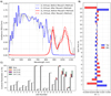Fig. 4 Example of steps in the calibration method for Cell A. A) Virtual lamps at k = 15. Solid lines show EI, EII of the base spectrum, whilst dashed lines show the spectrum after applying Meusel’s method. B) Mismatch factors of EMeusel,k for k∊[1, m–1]. kbest is the best splitting as it shows the lowest deviation. C) Change in {α} after calibration for Cell A, B, and C.

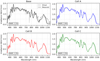Fig. 5 Virtual and measured spectrum for base and calibrated spectra.

4 Discussion

The method described above is effective but subject to several limitations. First, when implementing Meusel’s method (Sect. 2.3), the multiplication of the A from the two virtual lamps with the base coefficients α is unconstrained, which can result in ${\alpha }^{\text{Meusel}\mathrm{,}k}>1$ (Eq. (4)). In such cases, the values are bounded to the range [0, 1]. For Cells A, B, and C, LED 17 required bounding to 1 (Appendix, Tab. A1), which may explain why the ideal condition of Z = 1.00 was not achieved, as the truncated irradiance from LED 17 was not compensated after bounding. Compensation of this truncated irradiance using adjacent LEDs is a direction for future work.

Furthermore, all spectral measurements were performed in flash mode, and these measurements are assumed to be the stable representations of both E_j during characterization and E_sim during calibration and measurement. This assumption may not hold true, especially for applications requiring prolonged, steady illumination, such as the stabilized current-voltage characterization needed for perovskite-based devices [3]. Stabilized measurements were not taken as the solar simulator used in this study was equipped with a cooling system designed for flash measurements. This cooling system was insufficient to sustain AM1.5G simulation for extended periods. If operated continuously, the solar simulator temperature increases until its operational threshold is reached, before spectral stabilization occurs [5].

5 Conclusion

This study outlines a calibration method for multi-LED solar simulators used in the characterization of tandem solar cells, supported by an open-source code implementation. The method was validated using three perovskite-silicon tandem devices, resulting in spectral mismatch factors within 1±0.05 and matching factors within 1±0.03, meeting the requirements of the IEC 60904-1-1 standard. The effect of the calibration on the spectral shape was observed and explained. The method’s limitations are also discussed. The method and provided code are intended to offer a practical and accessible approach for laboratories to calibrate their multi-LED solar simulators for tandem devices.

Acknowledgments

The authors would like to thank and acknowledge Hou group for providing tandem solar cell samples.

Funding

This work was supported by the Solar Energy Research Institute of Singapore (SERIS) at the National University of Singapore (NUS). SERIS is supported by NUS, the National Research Foundation Singapore (NRF), the Energy Market Authority of Singapore (EMA) and the Singapore Economic Development Board (EDB). The author AB acknowledges financial support from EDF in the framework of the research and teaching Chair 'Sustainable energies' at École Polytechnique.

Conflicts of interest

The authors declare no conflicts of interest and have nothing to disclose.

Data availability statement

The calibration method can be found in https://github.com/Stella-Hdw/Multi-LED-Solar-Simulator-Calibration-for-Tandem-I-V. Further data can be provided upon request.

Author contribution statement

Conceptualization, A.B., Z.N., and S.H.; Methodology, A.B., Z.N., S.H., and Y.J; Software, A.B., Z.N., S.H.; Validation, A.B., Z.N., and S.H.; Formal Analysis, A.B., Z.N., and S.H.; Investigation, A.B., Z.N., and S.H.; Resources, S.H., Y.J., and C.K.; Data Curation A.B., Z.N., and S.H.; Writing – Original Draft Preparation, A.B., Z.N., and S.H.; Writing – Review & Editing, S.H.; Visualization, S.H.; Supervision, C.K.; Project Administration, C.K.; Funding Acquisition, C.K.

References

Appendix

A.1 Meusel’s method

The method assumes two adjustable light sources, I and II, with adjustable power A_I and A_II which ranges from 0 to 1. The paper assumes: linear scaling of power to output spectrum, independence of the two light sources (e.g. no thermal crosstalk) (Eq. (3)) and additive independence of the photo-current. The photocurrent densities of the two sub-cells under E_ref, can be calculated by:

$$J_{\text{top/bot}}^{\text{ref}}={\displaystyle {\int }_{{\lambda }_{\text{min}}}^{{\lambda }_{\text{max}}}}{E}_{\text{ref}}(\lambda )S{R}_{\text{top/bot}}(\lambda )d\lambda$$(A.1)

The photocurrent densities $J_{\text{top/bot}}^{\text{ref}}$ of the sub-cells measured under simulated light with relative spectra e_I(λ) and e_II(λ) are:

$$J_{\text{top/bot}}^{\text{sim}}=A_{\text{I}}{\displaystyle {\int }_{{\lambda }_{\text{min}}}^{{\lambda }_{\text{max}}}}{\text{SR}}_{\text{top/bot}}(\lambda )e_{\text{I}}(\lambda )d\lambda +A_{\text{II}}{\displaystyle {\int }_{{\lambda }_{\text{min}}}^{{\lambda }_{\text{max}}}}{\text{SR}}_{\text{top/bot}}(\lambda )e_{\text{II}}(\lambda )d\lambda$$(A.2)

The relative spectra e_I,e_II can be considered as the maximum spectral irradiance of the lamps, when A_II = 1. To achieve equal photo-current generation in the sub-cells under the simulated spectrum compared to the reference spectrum:

$$J_{\text{top}}^{\text{ref}}=J_{\text{top}}^{\text{sim}}\mathrm{,}\hspace{1em}{J}_{\text{bot}}^{\text{ref}}=J_{\text{bot}}^{\text{sim}}$$(A.3)

This system of equations can be rewritten as a matrix equation AX = B, and solved given the inversibility of A:

$$\left[\begin{array}{cc}{\displaystyle {\int }_{{\lambda }_{\text{min}}}^{{\lambda }_{\text{max}}}}{e}_I(\lambda ){\text{SR}}_{\text{top}}(\lambda )d\lambda & {\displaystyle {\int }_{{\lambda }_{\text{min}}}^{{\lambda }_{\text{max}}}}{e}_{II}(\lambda ){\text{SR}}_{\text{top}}(\lambda )d\lambda \\ & \\ {\displaystyle {\int }_{{\lambda }_{\text{min}}}^{{\lambda }_{\text{max}}}}{e}_I(\lambda ){\text{SR}}_{\text{bot}}(\lambda )d\lambda & {\displaystyle {\int }_{{\lambda }_{\text{min}}}^{{\lambda }_{\text{max}}}}{e}_{II}(\lambda ){\text{SR}}_{\text{bot}}(\lambda )d\lambda \end{array}\right]\left[\begin{array}{c}{A}_I\\ \\ A_{II}\end{array}\right]=\left[\begin{array}{c}{\displaystyle {\int }_{{\lambda }_{\text{min}}}^{{\lambda }_{\text{max}}}}{\text{SR}}_{\text{top}}(\lambda )E_{\text{ref}}(\lambda )d\lambda \\ \\ {\displaystyle {\int }_{{\lambda }_{\text{min}}}^{{\lambda }_{\text{max}}}}{\text{SR}}_{\text{bot}}(\lambda )E_{\text{ref}}(\lambda )d\lambda \end{array}\right]$$(A.4)

$$X=A^{-1}B$$(A.5)

A_I and A_II are parameters to adjust the intensity of each light.

$$E_{\text{I}}=A_I{e}_I(\lambda )=A_I{\displaystyle \sum _{i=1}^k}{\alpha }_i{e}_i(\lambda )\mathrm{,}\hspace{1em}{E}_{\text{II}}=A_{\text{II}}{e}_{\text{II}}(\lambda )=A_{\text{II}}{\displaystyle \sum _{j=k+1}^m}{\alpha }_j{e}_j(\lambda )$$(A.6)

A.2 Relating linear and non-linear LED control parameters

The calibration procedure requires translating the ideal linear control parameters from Meusel’s method into control parameters that account for LED non-linearity. Meusel’s method calculates coefficients ${\alpha }_j^{\text{Meusel}\mathrm{,}k}$ under the assumption of linear intensity control:

$${\alpha }_j^{\text{Meusel}\mathrm{,}k}=\{\begin{array}{cc}{A}_{\text{I}}{\alpha }_j^{\text{base}}\mathrm{,}& \text{for}\hspace{1em}j\le k\\ A_{\text{II}}{\alpha }_j^{\text{base}}\mathrm{,}& \text{for}\hspace{1em}j>k\end{array}$$(A.7)

This implies an ideal spectral response $E_j^{\text{linear}}(\lambda )={\alpha }_j^{\text{linear}}{e}_j(\lambda )$, where e_j(λ) represents the spectrum at maximum power. However, thermal effects cause significant deviation from this linear relationship. As mentioned in Section 3.2.1, the actual spectral output E_j(α_j) is determined empirically through linear interpolation of pre-characterized spectra measured at ${\alpha }_j\in \left\{\mathrm{0.1,0.2,...,1.0}\right\}$ [7]. To bridge this discrepancy, we define the normalized total irradiance:

$$\langle {\alpha }_j\rangle =\frac{{\displaystyle \int }{E}_j({\alpha }_j)d\lambda }{{\displaystyle \int }{e}_{j}d\lambda }$$(A.8)

which serves as an empirical measure of actual LED output. For the ideal linear case:

$$\langle {\alpha }_j^{\text{linear}}\rangle =\frac{{\displaystyle \int }{\alpha }_j^{\text{linear}}{e}_{j}d\lambda }{{\displaystyle \int }{e}_{j}d\lambda }={\alpha }_j^{\text{linear}}$$(A.9)

The relationship between the target linear parameter and required physical parameter is characterized by a fifth-degree polynomial P_j (Fig. A.1):

$${\alpha }_j=P_j({\alpha }_j^{\text{linear}})$$(A.10)

where P_j is determined empirically for each LED through np.polyfit. The calibrated control parameters are therefore obtained through:

$${\alpha }_j^{\text{calib}.}=P_j\left(min(\mathrm{1,}{\alpha }_j^{\text{Meusel}\mathrm{,}k})\right)$$(A.11)

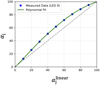Fig. A.1 Polynomial characterization of LED 9’s non-linear response, showing the relationship between input control parameter (αlinear) and normalized output irradiance (〈αj〉).

This approach is similar to the method in [1], but uses normalized irradiance rather than reference solar cell current for the polynomial correction. The complete set of polynomial coefficients for all LEDs used in the study is provided in the Appendix, Table A.3. The choice of using a fifth-degree polynomial came from evaluating a good fit of polynomials from degree 1 to 8 (with the fifth order achieving R² = 1.0000). The average R² from the polynomial fitting across LEDs can be seen in Table A.4.

All Tables

All Figures

	Fig. 1 Spectral irradiance of the LEDs at maximum power of the solar simulator used.
In the text

	Fig. 2 EQE of reference solar cells (grey), and tandem solar cells (A in orange, B in purple, C in green).
In the text

	Fig. 3 Reference spectrum (AM1.5G) (in grey), base spectrum (in black) and calibrated spectra for Cell A (orange), B (purple), and C (green).
In the text

	Fig. 4 Example of steps in the calibration method for Cell A. A) Virtual lamps at k = 15. Solid lines show EI, EII of the base spectrum, whilst dashed lines show the spectrum after applying Meusel’s method. B) Mismatch factors of EMeusel,k for k∊[1, m–1]. kbest is the best splitting as it shows the lowest deviation. C) Change in {α} after calibration for Cell A, B, and C.
In the text

	Fig. 5 Virtual and measured spectrum for base and calibrated spectra.
In the text

	Fig. A.1 Polynomial characterization of LED 9’s non-linear response, showing the relationship between input control parameter (αlinear) and normalized output irradiance (〈αj〉).
In the text

References

- ITRPV, International Technology Roadmap for Photovoltaic (ITRPV): Publication of the 6th Edition. Technical report, International Technology Roadmap for Photovoltaic (ITRPV), (2024) [Google Scholar]
- H. Li, W. Zhang, Perovskite tandem solar cells: from fundamentals to commercial deployment, Chem. Rev. 120, 9835 (2020) [Google Scholar]
- T. Song, D.J. Friedman, N. Kopidakis et al., How should researchers measure perovskite-based monolithic multijunction solar cells’ performance? a calibration lab’s perspective, Sol. RRL 6, 2200800 (2022) [Google Scholar]
- IEC 60904-1-1, Photovoltaic devices –Part 1-1: Measurement of current-voltage characteristics of multi-junction photovoltaic (PV) devices, 2017 [Google Scholar]
- D. Chojniak, M. Schachtner, S.K. Reichmuth, A.J. Bett, M. Rauer, J. Hohl-Ebinger, A. Schmid, G. Siefer, S.W. Glunz, A precise method for the spectral adjustment of LED and multi-light source solar simulators, Prog. Photovolt.: Res. Appl. 32, 372 (2024) [Google Scholar]
- T. Song, C. Mack, J. Brewer, J.F. Geisz, R. Williams, D.J. Friedman, N. Kopidakis, Closing the Accuracy Gap in Tandem Photovoltaic Testing: An Accessible and Efficient Spectral Tuning Method Using LED-Based Simulators for Research Laboratories and Industry, PRX Energy 4,033005 (2025) [Google Scholar]
- E. Technology, https://enlitechnology.com/product/reference-cell-src-2020/ [Google Scholar]
- M. Mackiewicz, S. Crichton, S. Newsome, R. Gazerro, G.D. Finlayson, A. Hurlbert, Spectrally tunable LED illuminator for vision research, Conf. Colour Graph. Imaging Vis. 6, 372 (2012) [Google Scholar]
- S. Crichton, S. Newsome, R. Gazerro, G. Finlayson, A. Hulbert, Spectrally tunable LED illuminator for vision research, in CGIV 2012 Final Program and Proceedings (2012) [Google Scholar]
- J.A. Nelder, R. Mead, A simplex method for function minimization, Computer J. 7, 308 (1965) [Google Scholar]
- M. Meusel, R. Adelhelm, F. Dimroth, A.W. Bett, W. Warta, Spectral mismatch correction and spectrometric characterization of monolithic III–V multi-junction solar cells, Progress in Photovoltaics: Research and Applications 10, 243 (2002) [Google Scholar]
- International Electrotechnical Commission (IEC), Photovoltaic devices - part 9: Classification of solar simulator characteristics (IEC Standard 60904-9, 2020) [Google Scholar]
The assumption of this definition is discussed in Section 3.3.
Cite this article as: Antoine Bourgeois, Zoltan Nicot-Senneville, Stella Hadiwidjaja, Jiayi Ye, Kwan Bum Choi, Accessible spectral calibration of multi-LED solar simulators for tandem I–V measurement, EPJ Photovoltaics 17, 19 (2026), https://doi.org/10.1051/epjpv/2026008