| Issue |
EPJ Photovolt.
Volume 17, 2026
Special Issue on ‘EU PVSEC 2025: State of the Art and Developments in Photovoltaics', edited by Robert Kenny and Carlos del Cañizo
|
|
|---|---|---|
| Article Number | 11 | |
| Number of page(s) | 19 | |
| DOI | https://doi.org/10.1051/epjpv/2025027 | |
| Published online | 25 February 2026 | |
https://doi.org/10.1051/epjpv/2025027
Original Article
Standardized assessment of PV array simulators
1
Bern University of Applied Sciences (BFH), School of Engineering and Computer Science (TI), Institute for Energy and Mobility Research (IEM), Laboratory for Photovoltaic Systems (PV-Lab), Jlcoweg 1, 3400 Burgdorf, Switzerland
2
Austrian Institute of Technology (AIT), Center for Energy, Power and Renewable Gas Systems, Giefinggasse 2, 1210 Vienna, Austria
3
Fraunhofer Institute for Solar Energy Systems ISE, Heidenhofstr. 2, 79110 Freiburg, Germany
* e-mail: This email address is being protected from spambots. You need JavaScript enabled to view it.
Received:
18
July
2025
Accepted:
3
December
2025
Published online: 25 February 2026
Abstract
PV array simulators are devices for PV and PV battery inverter testing. To ensure that these devices operate correctly and can realistically simulate PV modules and PV arrays, a test procedure for the assessment of PV array simulators has been developed and is presented in this paper. This procedure helps testing laboratories to evaluate PV array simulators and leads to more uniform test conditions. Furthermore, it assists developers of such simulators in understanding the requirements, enabling them to optimize and test their devices accordingly. The proposed test series includes three phenomenological observations, in which the interaction between the PV array simulator and a randomly selected PV inverter is tested. Subsequently, three potentially standardisable tests are proposed in which certain properties, such as the accuracy and frequency response of the PV array simulators are tested and evaluated.
Key words: PV array simulator assessment / solar array simulator evaluation / photovoltaic inverter testing / I–V curve emulating / SAS quality
© T. Zwahlen et al., Published by EDP Sciences, 2026
 This is an Open Access article distributed under the terms of the Creative Commons Attribution License (https://creativecommons.org/licenses/by/4.0), which permits unrestricted use, distribution, and reproduction in any medium, provided the original work is properly cited.
1 Introduction
The use of distributed renewable energy sources keeps increasing globally. Solar photovoltaics (PV) will account for around 80% of the global increase in renewable power capacity over the next 5 yr, with its expansion taking place in a context of grid integration challenges. The amount of installed renewable power is forecast to more than double by 2030 [1].
Because distributed energy resources (DERs) such as PV and wind systems are predominantly inverter-based, correct functionality of PV inverters is essential for the expansion of renewable energy. Modern PV inverters are not just passive, they actively contribute to grid stability with functions such as voltage regulation, bulk system control and other grid services [2]. This necessitates rigorous and extensive testing procedures to validate their performance. Several standards already exist for inverters, including how they are to be tested — for example, “EN50530 Overall Efficiency of Grid Connected PV Inverters” [3], the “BVES/BSW Efficiency Guideline for PV Storage Systems” [4], and various grid-code standards. In addition to existing test standards for the grid connection (e.g. [5–7]), it will become increasingly important to precisely characterise the behaviour of PV inverters that provide grid support [8].
To test inverters, laboratories need several devices such as alternating current (AC) grid simulators and PV array simulators (PVAS). These devices need to correctly mimic the behaviour of a power grid or a series-connected string of photovoltaic modules with sufficient dynamics, including direct current (DC) ripple caused by inverters [9,10]. As an overview and introduction to the topic, reference [11] provides a review of various PV array simulator architectures, including their advantages, disadvantages and their effectiveness in replicating the current-voltage (I-V) characteristics of real PV modules. Requirements for PV array simulators can be derived from relevant test standards. Additionally, a technical specification from the International Electrotechnical Commission (IEC) provides guidelines for the electrical performance of a DC source intended for use as PV array simulators [12]. However, there are currently no established guidelines on how the PV array simulators themselves should be tested or evaluated. Moreover, the existing specifications are formulated rather vaguely, placing much of the interpretive responsibility on the testing laboratories.
To maintain efficiency of PV systems, it is crucial to understand how PV modules behave under various conditions. With technological advancement in PV array simulators, PV performance under more realistic environmental conditions can be analysed and thus lead to more reliable predictions. This further underlines the need for rigorous and standardized testing and evaluation of PV array simulators.
To date, only a single publication has specifically addressed the testing and assessment of PV array simulators [13]. This study outlines three test procedures and evaluates two commercial PV array simulators. The first test procedure (Steady-State Behaviour of SAS) closely resembles the phenomenological observation 1: I-V Curve Instability (Sect. 2.3.1) in the present paper. The remaining two test methods focus on the dynamic performance of PV array simulators, examining their behaviour under changing load conditions and during curve transitions, such as those caused by irradiance fluctuations. The study concludes that commercial PV array simulators possess significant limitations and inaccuracies, which compromise their reliability. Since the ability to quickly identify the maximum power point after a change in the I-V curve is essential for the efficiency of model-based MPPT algorithms, these limitations are especially critical to evaluate the latter [13].
Recent tests for PV battery inverters at AIT showed that some state-of-the-art PV array simulators produce stronger DC-ripple or oscillations than would be expected. One PV simulator, tested with a commercially available PV inverter, produced such strong oscillations that MPPT efficiency could not be evaluated correctly from the PV array simulator. It displayed incorrect values exceeding 100% efficiency.
To assess whether PV array simulators meet the requirements of testing laboratories, the Laboratory for Photovoltaic Systems of the Bern University of Applied Sciences (BFH) and the Power and Renewable Gas Systems research group of the Austrian Institute of Technology (AIT) initiated the development of a dedicated test procedure to evaluate PV array simulators. The Fraunhofer Institute for Solar Energy Systems (Fraunhofer ISE) later joined the project, contributing additional expertise based on its familiarity with the challenges related to PV array simulators. This paper presents the developed test procedure and includes some anonymized results from evaluations of PV array simulators.
2 Test method and background
Array simulators emulating the I-V curve of a PV array are usually based on digital switching power supplies without a linear output stage. Their small-signal characteristics result from the performance of the power electronics and control software. The array simulators tested in this paper exhibit slower dynamic behaviour compared to real PV modules, particularly when used in conjunction with PV inverters. The current output does not adjust instantaneously to changes in input voltage, resulting in a delayed emulation of real PV dynamics that can impair accurate inverter testing and maximum power point tracking (MPPT) performance. In conjunction with PV inverters, this often leads to undesirable behaviour such as oscillations between the array simulators and the PV inverter.
The existing test criteria proposed for PV array simulators are considered necessary by the authors, but not sufficient to ensure realistic inverter operation − particularly in the case of grid support mode. Without dedicated and appropriate individual tests, it remains uncertain whether an array simulator is compatible with a particular PV inverter or not. However, the following can help identify whether undesirable phenomena are likely to occur when using a particular array simulator during inverter testing.
Wo categories are proposed:
Phenomenological observations (can only be standardised to a limited extent): These observations quickly reveal problems in the test environment, with their extent varying greatly from simulator to simulator. In Phen 2 and Phen 3, the array simulator is tested together with a PV inverter. The choice of inverter has significant influence on the test results. Due to the non-repeatability of the procedures, no pass-fail criteria are defined.
Standard tests: In these tests, the array simulator is operated under defined conditions and without a PV inverter. Pass-fail criteria are defined for these tests.
While the phenomenological observations are meant to showcase different issues arising when using PV array simulators in general, and especially in combination with an inverter, the standard tests are meant to classify a particular PV array simulator via pass-fail criteria. In Table 1 an overview of the categories and their respective sub-categories can be found.
Overview of the proposed tests and observations for evaluating array simulators.
2.1 Measurement setup
This section briefly describes the measurement setups used for evaluating PV array simulators. In total, four different setups are used, all of which use similar or identical measurement equipment. For tests that focus on accuracy (e.g. Std 3), a high-precision power analyser should be used to measure both voltage and current, and to calculate power. If the analyser also provides high-resolution raw measurement values (>50 kHz), these values can also be used for further analysis. Otherwise, an additional oscilloscope with appropriate measuring probes should be integrated into the setup.
In measurement setup 1, the PV array simulator is loaded using a DC power supply capable of sinking power. The power supply should be powerful enough to work in full range of the operating points as described in Section 2.1.1. Additionally, it must be able to run simple programmed functions, such as ramp profiles. Figure 1 presents a block diagram of the measurement setup 1.
Measurement setup 2 involves connecting the simulator to various randomly selected PV inverters. At least two different inverters are recommended. The PV array simulators under assessment should be tested using the same inverter devices as reference units to ensure comparability. A block diagram corresponding to Measurement setup 2 is shown in Figure 2.
As in measurement setup 1, measurement setup 3 contains a DC power supply with sink functionality. Additionally, an AC power supply is added to load the PV array simulator with superimposed dynamic signals. It is also possible to provide the DC load and the AC superimposition using a single device, if it allows a corresponding modulation. Figure 3 shows the block diagram for measurement setup 3.
Measurement setup 4 is the simplest case. Since changes in irradiance directly correspond to changes in short-circuit current [14], some observations regarding irradiance variation can most easily be made with the output of the PV array simulator short-circuited. Figure 4 shows measurement setup 4 as a block diagram, although voltage measurement is not actually required in this case.
For all measurement setups, a list of the exact devices used for the measurements conducted within the scope of this study can be found in Appendix A.
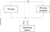 |
Fig. 1 Measurement setup 1: Block diagram of a PV array simulator loaded with a bidirectional DC power supply. |
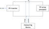 |
Fig. 2 Measurement setup 2: Block Diagram of a PV array simulator loaded with a common PV inverter. |
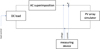 |
Fig. 3 Measurement setup 3: Block Diagram of a PV array simulator loaded with a bidirectional DC power supply and an additional AC source to superimpose an alternating voltage. |
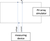 |
Fig. 4 Measurement setup 4: Block diagram of a PV array simulator with short-circuited output. |
2.1.1 Operating points
For all tests with a static I-V curve, the PV array simulator should be parametrised as described in this section. A characterisation according to EN50530 with cell type crystalline silicon (cSi) cell type [3] should be used in each case, to ensure comparability, to match the behaviour of most real PV modules and to ensure functionality with inverter electronics, which are usually tuned for c-Si. For the tests, four different operating points (OP) are used with the parameters described in Table 2. The absolute parameters are chosen to test PV array simulators with a maximum output voltage of 1500 V. OP1 was chosen to represent a single PV module. The value of OP4 (1000 V @MPP) was chosen at this VMPP to represent a realistic yet large PV system. Because the array simulators have a maximum output voltage of 1500 V, the open-circuit voltage can still safely be reached, and the full I-V-curve can still be traced by an inverter. Next, OP2 was chosen to test the simulators at a rather low voltage, and lastly OP3 was chosen in between to represent an average, medium sized PV system, such as a roof-mounted array of modules. Furthermore, the four operating points cover a large portion of the simulator's output range.
Since these absolute operating points are rigid, an additional method is proposed in Appendix A to adapt the values for PV array simulators with output ratings differing from the chosen maximum output voltage of 1500 V. In the following sections, only the absolute operating points as defined in Table 2 were used.
Operating point parameters for tests with static I-V curve.
2.1.2 PV inverters used in setup 2
In measurement setup 2, at least two PV inverters are used as reference devices for selected tests. The specific devices employed are listed in Table 3. As the authors do not consider the results as indicative of inverter quality, the devices have not been anonymized.
PV inverter used in measurement setup 2.
2.2 Devices under test
The test procedures proposed in this paper were developed in parallel with the evaluation of PV array simulators. The purpose of this study is to develop a suitable testing procedure to test and judge PV array simulators and to ascertain possible problematic behaviours in PV array simulators, not to scrutinize and categorize individual simulators or manufacturers. The development of this procedure required a lot of refinement during the testing campaign to optimize the tests themselves. Most of the devices were examined at the Laboratory for Photovoltaic Systems at BFH, with some tests also conducted at the Austrian Institute of Technology (AIT). A lot of the devices were provided by distributors or manufacturers and were therefore only available for a limited amount of time. For most refined and finalized tests, only a few of the PV array simulators were still available to examine. Thus, not all tests were conducted on the same number of simulators. Table 4 lists all PV array simulators for which measurement data was included in the analysis. The table also indicates the institute at which each device was tested, along with its respective device type. Regarding the device type, a distinction is made between bidirectional and unidirectional simulators. Unless otherwise stated in the table, the simulators — both unidirectional and bidirectional — employ nonlinear switched-mode power supplies.
In the following sections, the PV array simulators are referred to anonymously to protect the interests of manufacturers who supplied equipment for testing.
Furthermore, the following devices were used as additional reference devices in some of the tests. The two devices equipped with linear output stages were developed in-house at the respective institutes. For some tests, a real PV system is also used as a reference. These reference devices and real PV modules are specified in Table 5.
PV array simulators included in the tests.
PV array simulators and real PV modules included as reference devices in the tests.
2.3 Phenomenological observations
Test laboratories are familiar with the challenge: unexpected phenomena can occur with every new test and Device Under Test (DUT). The causes do not necessarily lie within the DUT itself but may also result from interactions between the DUT and the laboratory infrastructure. In the case of PV array simulators, the authors have observed several phenomena of that type. Some of them can be specifically induced with simple setups. There are no strict pass-fail criteria; instead, they should be used to scrutinise the accuracy and validity of subsequent practical tests.
The following three sections describe the known phenomena and simple ways to induce them.
2.3.1 Phen 1: I-V curve instability
One phenomenon that can occur with PV array simulators is instability at operating points on the I-V curve. The instabilities are highly dependent on the behaviour of the load at the output. Furthermore, not all instabilities occur along the full I-V-curve, with some only visible in certain voltage ranges. Therefore, evaluation using a standardised test procedure is difficult. However, indications of instabilities are already partially visible in the live preview of the PV array simulator's operating software (see Fig. 5, which shows an example of such a live preview with oscillations).
Such instabilities can usually be caused by slowly sweeping over the entire I-V curve with a bidirectional DC power supply (measurement setup 1 as described under 2.1). In the proposed test, the PV array simulator is operated at each operating point described under 2.1.1. The load is then increased from 0 V to the open-circuit voltage (UOC) in 5 s and then reduced back to 0 V within the next 5 s. This semi-static load varies slowly enough to avoid subjecting the simulator to rapid dynamic changes, which ensures that oscillations are not intentionally triggered and that distortions of the I-V curve due to secondary effects are avoided. Figure 6 shows how the measurement data should look, if no instabilities occur. The data in the figure was calculated according to the I-V curve model as described in EN50530 [3] in MATLAB [15]. The calculation is based on the settings for OP3 (see Sect. 2.1.1).
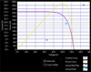 |
Fig. 5 Live preview (screenshot) of a PV array simulator operating software, running at an unstable operating point. The blue crosses, marking the minimum and maximum values, indicate strong oscillations around the operating point on the I-V curve. |
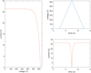 |
Fig. 6 Theoretical simulation result of an I-V curve instability test without any instabilities. Left: X-Y plot corresponding to the I-V curve. Right: time series of voltage (top in blue) and current (bottom in orange). The calculation follows an I-V model according to EN50530. |
2.3.2 Phen 2: Current ripple
Another localized issue lies in a high level of current ripple, generated by some PV array simulators at their output. Such ripple can interfere with the MPP tracking function of the inverter and lead to inaccuracies in measurements. Depending on the inverter connected to the PV array simulator and the load, the magnitude of the ripple varies greatly.
Figure 7 shows a segment of the measured current during an MPP tracking efficiency measurement according to EN50530 [3]. The red trace represents the raw current measurement sampled at 100 kHz, while the blue trace displays a 10 ms moving average of the raw current.
Current ripple (as can be seen in Fig. 7) can be reduced by connecting an inductance in series to the simulator's output. However, this in turn changes behaviour in other areas, e.g. in dynamics.
To compare current ripples for different PV array simulators, Phen 2 consists of a partly dynamic MPP tracking efficiency measurement according to EN50530, using at least two different inverters (measurement setup 2, see Sect. 2.1). The part of the dynamic MPPT efficiency measurement which was used is limited to the last line of Table B.3 in EN50530 [3]. The pattern is obtained based on Figure 8 and the parameters are given in Table 6. GSTC refers to the rated DC power of the inverter.
Ripples in the higher frequency range (>20 kHz) are caused by the switching frequency of the DC input stage of the PV inverter. Since frequencies at this level are expected to have a minor influence on measurement reliability, they can be filtered out. To filter them out, a fourth-order low-pass filter with a cutoff frequency of 10 kHz was used.
To compare the current ripple, a peak-to-peak calculation over 200 ms of the filtered signal is used. The comparison is made only for the high and for the low-level static area in the current pattern (3.8 A and 12.0 A in Fig. 7) and is expressed relative to the current setpoint at each respective level.
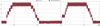 |
Fig. 7 Part of an MPP tracking efficiency measurement with raw current values (red) and averaged current values (blue). Screenshot taken from Dewetron power analyser [16]. |
2.3.3 Phen 3: MPPT efficiency difference
This phenomenological observation is not based on one single specific phenomenon. The idea of this test is to determine, whether the measured MPPT efficiency of one specific inverter varies depending on the PV array simulator used. The measurement for this test can be combined with the current ripple test described under 2.3.2. It uses the same pattern, measurement setup, and the same two inverters as in Phen 2. The pattern is described under 2.3.2 and in Figure 8 and Table 6. Usually, this test is pre-implemented on the PVAS, and the simulators directly return the average of the MPPT efficiency over the whole test duration. The MPPT efficiency is calculated by dividing the measured power by the available power at the MPP. To obtain more information about the cause of deviations, it is recommended to supplement the measurements with an external power measurement.
2.4 Standard tests
While the phenomenological observations as described in the previous sections provide a general overview of the PV array simulator's behaviour, the following three tests focus on a more detailed and reproducible assessment of the simulators. These tests can be performed in a manner similar to standardised procedures and highlight the aspects in which a simulator deviates from the behaviour of real PV modules, as well as its suitability for specific inverter testing applications. The tests can either be carried out with pass/fail criteria or used as a basis for comparing and ranking different PV array simulators.
The following three sections describe the background of each test and explain how each one is conducted.
2.4.1 Std 1: MPP accuracy and drift
To calculate the MPPT efficiency of an inverter, the maximum power available at the output of the PV array simulator must always be known. The accuracy of the output maximum power is based on the accuracy of the current and voltage measurements used within the simulator. These measurements are also used for the internal calculation of the MPPT efficiency within the simulator. The following test is used to rate the accuracy of the delivered power.
For this purpose, the PV array simulator is loaded with an adjustable load as described in measurement setup 2 under 2.1. The test is conducted separately for operating points 1 to 4. After the PV array simulator output is enabled, the load is manually adjusted until the maximum power is reached. With this approach, an MPP tracking is carried out manually. Once the maximum power is reached, the output is averaged over a period of 1 min and compared with the commanded setpoint.
To additionally observe the drift during the warm-up phase of the PV array simulator, manual MPP tracking is repeated after the PV array simulator has been operated at the identified power for 10 min. The resulting power is again averaged over 1 min. The process of the whole test is illustrated as a flow chart in Figure 9.
The EN50530 standard [3] may serve as a basis for defining a pass/fail threshold for the test. According to Section A.1.2, a simulator used for testing in compliance with this standard must maintain a power deviation of less than 1% within the voltage range from 0.9 × VMPP to 1.1 × VMPP. Since the standard requires the devices to be warmed up before the start of the test, it is sufficient to assess accuracy after a total waiting time of 10 min. However, it is still valuable to understand the drift behaviour of a device during the warm-up phase.
This relatively large power deviation tolerance is often acceptable, particularly if the power measurement is affected by the same error, which then cancels out in the efficiency calculation. This applies in all cases where the PV array simulator itself supplies the measurement data and performs the efficiency calculation. Under increased accuracy requirements, limits that are ten times smaller also appear to be realistic. Provided that the MPP accuracy is below 0.1%, MPPT efficiencies of up to 99.9% can be determined based on external measurement data.
 |
Fig. 9 Flow chart illustrating the MPP accuracy and drift test procedure. |
2.4.2 Std 2: Frequency response
For various reasons, PV inverters may impose oscillations or rapidly changing load on a PV array simulator. A typical example is the 100 Hz ripple propagated from the AC side of single-phase inverters, as described in [1,3]. Also, three phase inverters can subject the PV array simulator to a ripple load — for example, during MPPT operation, which induces minor load fluctuations [12], during load adjustments under curtailed grid connection conditions, or even due to malfunctions in the inverter's current regulator.
To evaluate how a PV simulator responds to load variations as described above and whether it behaves similarly to a real PV array, the following test is conducted. Measurement setup 3 is used (see Sect. 2.1), and the test is performed for all operating points described in Section 2.1.1. The PV array simulator is continuously loaded by a DC load at the MPP. An AC signal with a peak-to-peak voltage amplitude of ±2% UMPP is superimposed onto the load. The frequency of the AC voltage signal is swept from 0 to 1000 Hz. During the increase of the frequency, the phase shift between voltage and current at the simulator's output is measured. According to the I-V characteristics of PV modules, the current should decrease when voltage increases, implying an expected phase shift of 180°.
Figure 10 illustrates a theoretical example of the current response to a 100Hz voltage ripple. To improve visibility, an increased amplitude of ±3% was used for this calculation.
As a criterion for passing the test, a maximum phase shift of 180° ± 30° is proposed up to a frequency of at least 150 Hz. A phase angle of 180° is taken as the reference because, on the I-V curve, an increase in voltage results in a decrease in current. This inverse relationship corresponds to a negative correlation and therefore a phase shift of 180°. A phase shift of 30° is considered significant; however, many laboratory measurements are still expected to be feasible—albeit with limitations—under such conditions. Since 100 Hz is a typical frequency for inverter-induced loading on the DC side, compliance with the maximum allowable phase shift is evaluated up to 150 Hz to provide an appropriate margin.
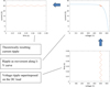 |
Fig. 10 Visualization of the theoretical impact of a 100 Hz voltage ripple on the current, generated by simulation. |
2.4.3 Std 3: Irradiance variation
In many tests, such as the determination of dynamic MPP tracking efficiency according to EN 50530, PV array simulators are required to follow an irradiance ramp. In most cases the simulators cannot continuously reproduce such linear ramps. Typically, power is adjusted in discrete steps at fixed time intervals.
A straightforward initial approach to evaluating this behaviour is to determine the smallest possible time interval. This approach provides an initial impression, but it does not quantify the impact of this behaviour. A more detailed assessment involves calculating the error between the excepted continuous ramp and the resulting current waveform effectively delivered by the PV array simulator under test. For this test, the irradiation profile according to EN50530 (see Sect. 2.3.2, Tab. 6, Fig. 8) shall be used again, but with n = 1 (meaning only one period) instead of n = 10. As irradiance changes correspond directly to the changes in short circuit current, the simulator can be tested with the output short-circuited, as described in measurement setup 4 under Section 2.1. The assessment is carried out based on the measured current. For the parameterization of the I–V characteristic, a short-circuit current of ISC = 10 A can be set. The voltage plays a subordinate role, since the test is performed under short-circuit conditions. However, an open-circuit voltage in the mid-range of the simulator's output appears to be reasonable.
Due to the discrete output steps, the error is distributed symmetrically around zero, which can be shown by calculating the mean bias error (MBE),

where  is the ith predicted value, yi is the ith observed value and n is the sample size. A negative mean bias error indicates an underestimation of the slope, whereas a positive mean bias error indicates an overestimation. Therefore, the root mean squared error (RMSE),

is calculated to evaluate the overall error. To allow comparison between PVAS devices tested at different short-circuit currents, the results can be further normalized to the maximum current.
3 Results and discussion
This chapter presents and discusses the results obtained from an exemplary test series involving several PV array simulators. The first three sections present the phenomenological observations, demonstrating the varying behaviour of different PV array simulators and highlights where unexpected responses arise.
The next three sections cover the results of the standardized tests. They illustrate the range of performance across a selection of devices.
3.1 Phen 1: I-V curve stability
Several of the tested PV array simulators exhibited unstable behaviour in their I-V characteristics. Figure 11 displays the recorded I-V curves of four devices (PVAS1, PVAS2, PVAS3 and PVAS6) across all four operating points. One can see that the magnitude of the oscillations and their occurrence across operating points vary greatly between simulators. For example, PVAS2 exhibits only minor oscillations, and only within the lowest voltage range, whereas PVAS1 starts oscillating heavily at a OP4. PVAS6 exhibits completely different behaviour: at low voltages, a clear instability can be seen around the MPP-Voltage and beyond at OP1 and OP2, while the simulator shows little to no oscillations at OP3. At the highest MPP-voltage (namely OP4), PVAS6 begins rapidly oscillating for voltages above the MPP-voltage.
For operating point 4, a second load was connected in series with the primary load to ensure full coverage of the voltage range. This configuration may influence the stability performance of the PV array simulators.
To illustrate the impact of oscillations on a real inverter, Figure 12 presents the PV current of the SMA inverter (see Tab. 3) during the startup process. The DC input was supplied by PVAS1. At approximately 13 s and 23 s, undesired oscillations are clearly visible.
In conclusion, these oscillations appear frequently, in different magnitudes and at different voltages for different simulators. One needs to take these into consideration when testing and using a PV array simulator. Because of the large differences in the range at which the oscillations occur and the severity thereof, one particular simulator might be completely fine at a certain operating point and noticeably unstable at another.
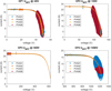 |
Fig. 11 Measured I-V curves of four PV array simulators at all four operating points. |
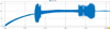 |
Fig. 12 PV current during startup of the SMA inverter supplied by PVAS1 (Dewetron screenshot). |
3.2 Phen 2: Current ripple
A current ripple assessment was conducted for the three devices PVAS1 to PVAS3. The upper part of Figure 13 shows the measured current waveform for a selected time segment. The filtered signal is shown, along with the derived minimum and maximum values. The lower part of the figure presents the resulting peak-to-peak current. A 4 s moving average is included, which serves to determine a reference value during periods of steady irradiance.
In Figure 14, the measured current ripple for PVAS1, PVAS2 and PVAS3 is presented, normalized to the average current at the respective power levels. The results highlight the significant influence of the connected inverter. When using the SMA inverter, all PV array simulators exhibit increased ripple levels. On the other hand, the test method itself proves to be meaningful, as lower ripple observed with one inverter correlates with lower ripple when using another inverter—indicating the method's consistency and transferability.
Although 3.5 A is considered a relatively low output current for PV array simulators, ripple values exceeding 20% are regarded as excessive and higher than would be expected from the inverter architecture. Even the best-performing simulator exhibits ripple close to 16%. Ripple levels remain significant even at other operating points or when switching out the inverter for a different one. Even with the less critical inverter in the exemplary test, ripple levels exceeding 10% were observed. Under more favourable conditions, particularly at higher power levels, at least two of the three simulators achieve ripple values below 5%.
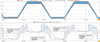 |
Fig. 13 Current waveform including filtered signal (top) and resulting peak-to-peak current (bottom) from the ripple test (Dewetron screenshot). |
 |
Fig. 14 Comparison of current ripple normalized to the average current at the respective power level. |
3.3 Phen 3: MPPT efficiency difference
As expected, the same test segment used to determine MPPT efficiency according to EN 50530 yields different results when conducted with different PV array simulators, even when using identical inverters. The result of this comparison among PVAS1, PVAS2, and PVAS3 using two different inverters is shown in Figure 15. One can clearly see large differences in the determined values. Furthermore, no uniform trend is evident; the inverter that performs best with PVAS1 differs from the one performing best with PVAS2. A more detailed look at the measurements themselves shows how these differences can arise. Therefore, Figure 16 presents the time evolution of the individual measurements.
The lower part of Figure 16 shows the time evolution of the MPPT efficiency determined by the three simulators. For comparison, three curves can be seen: Firstly, the efficiency calculated by an external measurement (externally measured power divided by setpoint power), secondly the efficiency provided by the PVAS itself, and lastly the efficiency calculated by an internal measurement (PVAS-internally measured power divided by setpoint power). For all devices, there are moments when the measured output power exceeds the theoretically available setpoint power, resulting in short-term MPPT efficiencies greater than 100%. The devices employ different strategies to handle this in the final efficiency calculation. While PVAS1 and PVAS2 additionally low-pass filter the reported MPPT efficiency, PVAS3 simply clips the values at 100%.
The time profile of the power measurement of PVAS1 (Fig. 16, top left) provides insight into the reason for the significantly lower efficiency measured with this array simulator. It is evident that this device is not capable of deterministically updating either the setpoint of the power at the MPP or its internally measured power. The varying update interval results in a substantial loss of accuracy. In addition, the long delay between a change in the setpoint and the corresponding change in the measured output power leads to large efficiency deviations during setpoint transitions. For example, when the setpoint is reduced, the output power may momentarily exceed the theoretically available power according to the PVAS model, resulting in MPPT efficiencies greater than 100%.
The differences between PVAS 2 and PVAS 3 are much smaller in the resulting overall MPPT efficiency; however, the time profiles show that this higher accuracy is achieved in different ways. Figure 17 shows a more detailed view of the power profiles of the two devices. PVAS 3 achieves higher accuracy through a faster update rate of the effectively available output power. Due to the faster response to setpoint changes, the differences between the prescribed and the actual power values are significantly reduced. PVAS2 has an output update rate that is just as low as that of PVAS1; however, because the device maintains precise timing, it can perform significantly more accurate calculations. It adjusts the setpoint curve such that it matches the actual output power. Moreover, this simulator accounts for the response time directly within the generated setpoint profile. As a result, the differences between the prescribed power and the measured output power are substantially reduced, even during setpoint transitions.
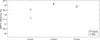 |
Fig. 15 Comparison of determined MPPT efficiencies using identical inverters and three different PV array simulators. |
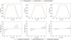 |
Fig. 16 Time evolution of the MPPT efficiency measurement of PVAS1 (left), PVAS2 (middle), and PVAS3 (right). The upper plots show the prescribed and the measured power, while the lower plots illustrate the resulting MPPT efficiency. |
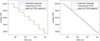 |
Fig. 17 Detailed time profile of the power for PVAS2 (left) and PVAS3 (right) during a power reduction in the MPPT efficiency measurement. |
3.4 Std 1: MPP accuracy and drift
The MPP accuracy was evaluated for three PV array simulators. Figure 18 shows example measurement data of one simulator. The blue curve indicates the externally measured power profile, while the orange curve represents the internally measured power. The red curve represents the MPP power provided by the PV array simulator (setpoint), and the purple curve is a 1 min moving average of the externally measured power. Manual MPP tracking was performed between 0–1.5 min and again at ∼12 min. The two highlighted measurement points in the figure are used for comparison.
Figure 19 presents the MPP accuracy test results for PVAS1 to PVAS3. The left-hand plot illustrates the deviations immediately after startup, while the right-hand plot shows the deviations after 10 min of operation across all four operating points. All three devices easily meet the requirement of a maximum deviation of 1% at OP 2 to OP 4 (shown in red in Fig. 19) as specified by EN50530. At OP 1, the error range is very large and extends beyond a deviation of more than 1%. This is due to the wide measurement range of the used power analyser, which leads to a large error when measuring such a small power level. Nevertheless, the additional requirement of a deviation below 0.1%, which would be necessary (as described under Sect. 2.4.1) to be able to measure MPPT efficiencies up to 99.9%, was not met by PVAS2. The other two simulators are within error range of said requirement. In addition to the result, Figure 19 includes the maximum inaccuracy of the measurement device used for the evaluation, shown as error bars [17].
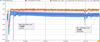 |
Fig. 18 MPP accuracy and drift measurement from PVAS3 on OP2 (Dewetron screenshot). |
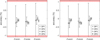 |
Fig. 19 MPP accuracy and drift measurement values after start up (left) and after loaded for 10 min at MPP (right) with error bars representing the uncertainty of the measurement device. |
3.5 Std 2: Frequency response
The frequency response was tested for a wide range of PV array simulators. While some of the simulators could be used on all operating points as described under Section 2.1.1, others were tested at slightly different voltages or could not be tested at certain points. For example, no measurements are available at operating point 4 for PVAS7 and PVAS8. Figure 20 provides an overview of the measured phase shift for all measured PV array simulators in the exemplary test series, categorized by OP1 to OP4. For comparison, the figure also includes comparable reference measurements from real PV modules roughly at OP1 to OP3 (RealPV). A comparative measurement at OP4 and exact voltage values for OP1 to OP3 were not possible due to infrastructure limitations (see also 2.2).
As shown in Figure 20, the frequency response of the tested devices varies significantly. Many simulators exhibit a considerable phase shift already at low frequencies, particularly at higher voltages (OP3 and OP4). A more detailed view is shown in Figure 21, where simulators with excessively large phase shifts have been omitted for improved readability. For comparison, the figure also includes data from two PV array simulators featuring linear output stages.
Figure 21 shows that only one tested PV array simulator with a non-linear output stage meets the requirement proposed in Section 2.4.2. This study does not include independent improvements of the devices, such as optimization of control parameters. However, manufacturers were given the opportunity to implement improvements themselves. Only one manufacturer was able to improve the behaviour. By setting a specific flag (SAS-BW = high), the bandwidth of the PV simulations on this device can be increased. Using this setting, the device was able to meet the requirement. The differences between the two flag states for this device are shown in Figure 22. While this device could not reach 1000 VMPP, the measurement for OP4 was taken at 800 VMPP. For this reason, the device is also not shown in the comparison in Figures 20 and 21.
The rather conservative criterion, namely a maximum phase shift of 180° ± 30° (up to a frequency of at least 150 Hz) already disqualifies many PV array simulators on the market.
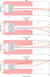 |
Fig. 20 Phase shift across frequency for all measured PV array simulators. |
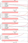 |
Fig. 21 Phase shift across frequency, showing better-performing PV array simulators and those with linear output stages as reference. |
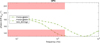 |
Fig. 22 Comparison of phase shift for PVAS4 with and without the SAS Bandwidth High setting. |
3.6 Std 3: Irradiance variation
The results presented below slightly differ from the suggested test procedure. Instead of the suggested ramp profile according to EN50530 (see Fig. 8, Tab. 6, Sect. 2.3.2), the parameters in Table 7 were used.
Due to different I-V characteristics programmed into the three simulators, the chosen value for the slope leads to differing values for the current. Figure 23, shows the measured current waveforms of the three simulators. The red trace represents the reference ramp used for error evaluation.
The reason for the mismatch in suggested and utilized test method is primarily pragmatic. Most of the devices used to develop and evaluate these tests were only available for a limited amount of time, and the suggested test method was devised after the measurements above had already been collected. Due to the restricted availability of the devices, the test could not be rerun using the proposed procedure. Nonetheless, the existing measurements illustrate the test's relevance, and the results of these three measurements are comparable. The homogeneity of the slope, despite its duration on the time axis being shorter than proposed, reveals how simulator-specific parameters, such as the update rate, influence the error.
Figure 24 presents the current error and the root mean square error (RMSE) calculated over the duration of each ramp. The consistent decrease in error during the upward ramp and increase during the downward ramp suggest that the devices deviate from the intended ramp profile, likely due to the discrete update interval and/or mismatched slopes.
Table 8 presents the normalized (n) RMSE and the normalized (n) MBE values, normalized to the current at maximum irradiance, for both the ramp-up and ramp-down phases of each PV array simulator.
To explain the differences in nRMSE, the smallest possible update rate for the simulators output was determined. This was carried out by applying an irradiation profile as described in Section 2.4.3. The duration of the individual steps was then determined from the measured current. If the steps were too short to be resolved using the standard-compliant irradiation profile, the ramp slope was increased until the step interval became discernible. In Figure 25, the minimal I-V curve update interval is shown for PVAS1 to PVAS8.
One can see that this update interval varies greatly from an overall minimum of 0.02 s for PVAS6 up to a full second for PVAS1, PVAS2 and PVAS5. The differences in nRMSE between PVAS1 and PVAS2 are minor, as the update rate of the irradiance is identical (1s) for both devices. PVAS8 exhibits a lower nRMSE, which can be attributed to its much shorter update rate of approximately 100ms, and thus to the better approximation of the continuous ramp profile.
The nMBE is noticeably smaller than the nRMSE. Especially for PVAS8, it is negligible compared to the nRMSE, meaning the simulator correctly implemented the intended slope without over- or underestimating it. The nRMSE can be explained by the discreteness of the update interval, even though for PVAS8 these errors are small, which can furthermore be seen when comparing the three devices in Figure 23. PVAS1 and PVAS2 show similar values for the nRMSE, as expected from their identical update rate. Their nMBE values vary slightly, with the exception of the ramp-up nMBE for PVAS1, which is roughly for times larger than the ramp-down value for the same simulator. When taking a closer look at Figure 24, this can be further explained: At the very beginning of the ramp-up process, a pronounced difference in intended and implemented slope can be seen for PVAS1. This outlier impacts the total MBE. Nonetheless, for all three devices, the nMBE is rather small compared to the nRMSE, meaning the discreteness of the update interval plays a bigger role in the overall error than their ability to correctly implement the slope. To ensure correct functionality of a PV array simulator and comparability of inverter tests run with different PV array simulators, the resolution on the time axis must be sufficiently precise to correctly implement the ramp profile according to EN50530.
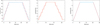 |
Fig. 23 Current profiles of PVAS1 (left), PVAS2 (middle), PVAS8 (right) with reference ramp (red). |
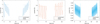 |
Fig. 24 Current error measured on PVAS1 (left), PVAS2 (middle), and PVAS8 (right), including the respective calculated RMSE value. |
Parameters used for the ramp profile for the irradiance test Std 3.
nRMSE and nMBE for three simulators during ramp-up and ramp-down.
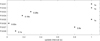 |
Fig. 25 Minimum I-V curve update interval measured for PVAS1 to PVAS8. |
4 Conclusion
This paper presents a test procedure for the assessment of PV array simulators, including results from three standardized tests and three phenomenological observations. Since the test methods were continuously developed during the assessment of eight different PV array simulators, not all tests include final results from every device. In some cases, results are available from only three simulators, which of course limits the generalisability of the findings. Still, especially the phenomenological tests underline that there exist unwanted effects of differing magnitudes across a range of simulators. Furthermore, the standardized tests present a way to categorize simulators and ensure their correct functionality and usability.
Most of the tests were conducted in the PV laboratory at the Bern University of Applied Sciences (BFH). In addition, two devices were tested by the Power and Renewable Gas Systems research group at the Austrian Institute of Technology (AIT) to verify the test procedure.
he results highlight substantial differences in output characteristics among the tested PV array simulators and demonstrate how these differences can influence inverter tests. For example, the observed differences in MPPT efficiency (Phen 3, Sect.3.3) raise concern about the reliability of this parameter as a comparative metric for inverters. The irradiance test (Std 3, Sect. 3.6) further underlines these findings and sets a quantitative threshold to evaluate a simulator's ability to correctly implement a linear ramp, such as the ramp according to EN50530 used to determine an inverters MPPT efficiency. The findings suggest that the type of PV array simulator used can significantly impact the measured efficiency, undermining direct comparability between inverters.
Particularly critical are I-V curve instabilities, especially considering the increasing use of power curtailment in inverter operation. For inverters known to the authors, this operating mode involves a deliberate voltage increase above the MPP − precisely the region where simulator oscillations frequently occur. This operational shift may affect future certification test protocols, as curtailed operation becomes more relevant. If PV array simulators exhibit instability under these conditions, test results may become invalid − or the tests might not be executable at all.
While the proposed test procedures offer a comprehensive framework for assessing PV array simulators, not all relevant behaviours have yet been covered. A known but unaddressed aspect is the synchronised control of multiple simulator outputs as required when supplying several MPP tracker inputs in parallel. The authors are aware that several PV array simulators offer only limited support for such operation, and time delays between outputs are commonly observed. A future test procedure update could address this issue by including a dedicated multi-channel synchronisation test.
Acknowledgments
A significant amount of the measurement data was obtained from PV array simulators that were provided by distributors or manufacturers for testing purposes. Their valuable cooperation and support are gratefully acknowledged.
Funding
This research received no external funding.
Conflicts of interest
BFH has a paid consulting agreement with a manufacturer aimed at improving their PV array simulator. However, the data used in this study was collected prior to this collaboration and is therefore not considered a conflict of interest. The other authors have nothing to disclose.
Data availability statement
For reasons of manufacturer confidentiality, the data associated with this article cannot be shared.
Author contribution statement
Conceptualization, Theo Zwahlen, Luciano Borgna, David Joss and Christof Bucher; Methodology, Theo Zwahlen, Luciano Borgna, David Joss and Christof Bucher; Validation, Christian Messner, Steffen Eyhorn and Michael Gafert; Data Curation, Theo Zwahlen and Michael Gafert; Writing − Original Draft Preparation, Theo Zwahlen; Writing − Review & Editing, Theo Zwahlen, David Joss, Lara Wenger, Christof Bucher, Christian Messner, Michael Gafert and Steffen Eyhorn; Visualization, Theo Zwahlen, David Joss; Supervision, Christof Bucher and Roland Bründlinger; Project Administration, Theo Zwahlen and David Joss.
References
- Executive summary − Renewables 2025–Analysis, IEA (n.d.). https://www.iea.org/reports/renewables-2025/executive-summary (accessed November 27, 2025) [Google Scholar]
- N. Ninad, E. Apablaza-Arancibia, M. Bui, J. Johnson, S. Gonzalez, R. Darbali-Zamora, C. Cho, W. Son, J. Hashimoto, K. Otani, R. Bründlinger, R. Ablinger, C. Messner, C. Seitl, Z. Miletic, I.V. Temez, J. Montoya, F. Baumgartner, C. Fabian, S. Kumar, J. Kumar, B. Fox, R. Brandl, R. Conklin, PV inverter grid support function assessment using open-source IEEE P1547.1 test package, in 2020 47th IEEE Photovoltaic Specialists Conference (PVSC) (2020), pp. 1138–1144. https://doi.org/10.1109/PVSC45281.2020.9300372 [Google Scholar]
- EN 50530:2010, Overall efficiency of grid connected photovoltaic inverters, 2010 [Google Scholar]
- BVES Bundesverband Energiespeicher Systeme, BSW-solar Bundesverband Solarwirtschaft, Efficiency guideline for PV storage systems, (n.d.). https://solar.htw-berlin.de/wp-content/uploads/Efficiency-guideline-for-PV-storage-systems-2.0.pdf (accessed June 30, 2025) [Google Scholar]
- SN EN 50549-1:2019(E) − DV-31964/1 − Electrosuisse, (n.d.). https:/shop.electrosuisse.ch/de/SN-EN-50549- 1_2019_E_ 48355.html (accessed July 16, 2025) [Google Scholar]
- SN EN 50549-2:2019+AC:2019(D) − DV-34426/1 − Electrosuisse, (n.d.). https://shop.electrosuisse.ch/de/SNEN-50549-2_2019_AC_2019_D_-54247.html (accessed July 16, 2025) [Google Scholar]
- SN EN 50549-10:2022(E) − DV-45035/1 − Electrosuisse, (n.d.). https://shop.electrosuisse.ch/de/SN-EN-50549-10_2022_E_-397612.html (accessed July 16, 2025) [Google Scholar]
- TC 82, Project: IEC 63409-6 ED1, IEC (International Electrotechnical Commission) (n.d.). https://www.iec.ch/dyn/www/f?p=103:38:601780107873093::::FSP_ORG_ID,FSP_APEX_PAGE,FSP_PROJECT_ID:1276,23,105972 (accessed July 16, 2025) [Google Scholar]
- R. Ayop, C.W. Tan, A comprehensive review on photovoltaic emulator, Renew. Sustain. Energy Rev. 80, 430 (2017). https://doi.org/10.1016/j.rser.2017.05.217 [Google Scholar]
- Spitzenberger & Spies, Necessity for high speed PV Simulators, n.d. www.spitzenberger.de/weblink/1005 (accessed January 24, 2025) [Google Scholar]
- J.P. Ram, H. Manghani, D.S. Pillai, T.S. Babu, M. Miyatake, N. Rajasekar, Analysis on solar PV emulators: a review, Renew. Sustain. Energy Rev. 81, 149 (2018). https://doi.org/10.1016/j.rser.2017.07.039 [Google Scholar]
- IEC TS 63106-2, Simulators used for testing of photovoltaic power conversion equipment − Recommendations − Part 2: DC power simulators (2022) [Google Scholar]
- V.M. Cavalcante Junior, R.C. Neto, E.J. Barbosa, F. Bradaschia, M.C. Cavalcanti, G.M.D.S. Azevedo, Evaluation of the effectiveness of solar array simulators in reproducing the characteristics of photovoltaic modules, Sustainability 16, 6932 (2024). https://doi.org/10.3390/su16166932 [Google Scholar]
- C. Bucher, Photovoltaikanlagen: planung, installation (Betrieb, 2. aktualisierte und erweiterte Auflage, Faktor Verlag, Zürich, 2025) [Google Scholar]
- The MathWorks Inc., MATLAB version: 24.2.0.2773142 (R2024b) Update 2, (2024). https://www.mathworks.com [Google Scholar]
- Dewetron, OXYGEN 7.5.1, (2025). https://www.dewetron.com/products/software/oxygen-software/ [Google Scholar]
- Dewetron, TRION3-1810M-POWER, (2025). https://ccc.dewetron.com/dl/5a8ac9b7-091c-4011-8803-5c5fd9c49a3c (accessed November 24, 2025) [Google Scholar]
Cite this article as: Theo Zwahlen, David Joss, Christian Messner, Christof Bucher, Luciano Borgna, Michael Gafert, Steffen Eyhorn, Lara Wenger, Roland Bründlinger, Standardized assessment of PV array simulators, EPJ Photovoltaics 17, 11 (2026), https://doi.org/10.1051/epjpv/2025027
Appendix A List of devices used for the measurements
List of measurements devices.
Relative operating points for simulators with differing output voltage
Since the absolute operating points in Table 2 are rigid, an additional method is proposed to adapt the values for PV array simulators with differing output ratings: OP 1 can be retained to represent a single module. For OP2 to OP4 the voltage VMPP can be set relative to the maximum output voltage of the PV array simulator VPVAS,MAX according to Table A2. For the operating point current, either the absolute current from Table 2 may be used, or the current can be scaled based on the relative power, as described in Table A2.
Operating point parameters for tests with static I-V curve, relative to the output specifications of the PV array simulator under test.
All Tables
PV array simulators and real PV modules included as reference devices in the tests.
Operating point parameters for tests with static I-V curve, relative to the output specifications of the PV array simulator under test.
All Figures
|
Fig. 1 Measurement setup 1: Block diagram of a PV array simulator loaded with a bidirectional DC power supply. |
| In the text | |
|
Fig. 2 Measurement setup 2: Block Diagram of a PV array simulator loaded with a common PV inverter. |
| In the text | |
|
Fig. 3 Measurement setup 3: Block Diagram of a PV array simulator loaded with a bidirectional DC power supply and an additional AC source to superimpose an alternating voltage. |
| In the text | |
|
Fig. 4 Measurement setup 4: Block diagram of a PV array simulator with short-circuited output. |
| In the text | |
|
Fig. 5 Live preview (screenshot) of a PV array simulator operating software, running at an unstable operating point. The blue crosses, marking the minimum and maximum values, indicate strong oscillations around the operating point on the I-V curve. |
| In the text | |
|
Fig. 6 Theoretical simulation result of an I-V curve instability test without any instabilities. Left: X-Y plot corresponding to the I-V curve. Right: time series of voltage (top in blue) and current (bottom in orange). The calculation follows an I-V model according to EN50530. |
| In the text | |
|
Fig. 7 Part of an MPP tracking efficiency measurement with raw current values (red) and averaged current values (blue). Screenshot taken from Dewetron power analyser [16]. |
| In the text | |
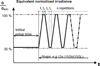 |
Fig. 8 Test sequence with a 30 % − 100 % ramp according to EN50530 [3]. |
| In the text | |
|
Fig. 9 Flow chart illustrating the MPP accuracy and drift test procedure. |
| In the text | |
|
Fig. 10 Visualization of the theoretical impact of a 100 Hz voltage ripple on the current, generated by simulation. |
| In the text | |
|
Fig. 11 Measured I-V curves of four PV array simulators at all four operating points. |
| In the text | |
|
Fig. 12 PV current during startup of the SMA inverter supplied by PVAS1 (Dewetron screenshot). |
| In the text | |
|
Fig. 13 Current waveform including filtered signal (top) and resulting peak-to-peak current (bottom) from the ripple test (Dewetron screenshot). |
| In the text | |
|
Fig. 14 Comparison of current ripple normalized to the average current at the respective power level. |
| In the text | |
|
Fig. 15 Comparison of determined MPPT efficiencies using identical inverters and three different PV array simulators. |
| In the text | |
|
Fig. 16 Time evolution of the MPPT efficiency measurement of PVAS1 (left), PVAS2 (middle), and PVAS3 (right). The upper plots show the prescribed and the measured power, while the lower plots illustrate the resulting MPPT efficiency. |
| In the text | |
|
Fig. 17 Detailed time profile of the power for PVAS2 (left) and PVAS3 (right) during a power reduction in the MPPT efficiency measurement. |
| In the text | |
|
Fig. 18 MPP accuracy and drift measurement from PVAS3 on OP2 (Dewetron screenshot). |
| In the text | |
|
Fig. 19 MPP accuracy and drift measurement values after start up (left) and after loaded for 10 min at MPP (right) with error bars representing the uncertainty of the measurement device. |
| In the text | |
|
Fig. 20 Phase shift across frequency for all measured PV array simulators. |
| In the text | |
|
Fig. 21 Phase shift across frequency, showing better-performing PV array simulators and those with linear output stages as reference. |
| In the text | |
|
Fig. 22 Comparison of phase shift for PVAS4 with and without the SAS Bandwidth High setting. |
| In the text | |
|
Fig. 23 Current profiles of PVAS1 (left), PVAS2 (middle), PVAS8 (right) with reference ramp (red). |
| In the text | |
|
Fig. 24 Current error measured on PVAS1 (left), PVAS2 (middle), and PVAS8 (right), including the respective calculated RMSE value. |
| In the text | |
|
Fig. 25 Minimum I-V curve update interval measured for PVAS1 to PVAS8. |
| In the text | |
Current usage metrics show cumulative count of Article Views (full-text article views including HTML views, PDF and ePub downloads, according to the available data) and Abstracts Views on Vision4Press platform.
Data correspond to usage on the plateform after 2015. The current usage metrics is available 48-96 hours after online publication and is updated daily on week days.
Initial download of the metrics may take a while.