| Issue |
EPJ Photovolt.
Volume 14, 2023
Special Issue on ‘WCPEC-8: State of the Art and Developments in Photovoltaics’, edited by Alessandra Scognamiglio, Robert Kenny, Shuzi Hayase and Arno Smets
|
|
|---|---|---|
| Article Number | 24 | |
| Number of page(s) | 24 | |
| Section | Modules and Systems | |
| DOI | https://doi.org/10.1051/epjpv/2023015 | |
| Published online | 04 August 2023 | |
https://doi.org/10.1051/epjpv/2023015
Regular Article
How cool is floating PV? A state-of-the-art review of floating PV's potential gain and computational fluid dynamics modeling to find its root cause
1
imec, Kapeldreef 75, Leuven, Belgium
2
EnergyVille, ThorPark 8310, Genk, Belgium
3
University of Hasselt, Martelarenlaan 42, Hasselt, Belgium
4
University of Leuven, Dept. of Electrical Engineering (ESAT), Leuven, Belgium
* e-mail: This email address is being protected from spambots. You need JavaScript enabled to view it.
Received:
1
July
2022
Received in final form:
1
March
2023
Accepted:
5
June
2023
Published online: 4 August 2023
Abstract
The noticeable rise in electricity demand, environmental concerns, and the intense land burden has led to installing PV systems on water bodies to create floating photovoltaic (FPV). Of all market niches, FPV is the one developing the fastest. Along with some of its well-documented merits comes a claim that FPV modules operate at a lower temperature than their ground-mounted counterparts (GPVs). This claim is essential due to the performance loss of PV modules at high operating temperatures. Some literature claims that FPVs are so well-cooled that they maintain around 10% higher efficiencies. However, this cooling is poorly quantified, and the root cause remains unclear in the industry. In this paper, an extensive review of all the latest published literature and white paper advertisements was analyzed. The gains in energy yield coming from different root causes range from 0.11% to 31.29%! This proves the point of lack of clarity of potential gain of FPV. The paper then analyses four possible explanations for this cooling effect and its root causes. The FPV performance parameters are isolated and systematically investigated through physics-based finite element modeling. The impacts of wind velocity, wind direction, water temperature, relative humidity, air temperature, proximity to water, tilt angle, and others are evaluated and explained. The outcomes dictate that FPV is cooled largely through wind convection. But the increase in efficiency is below the anticipated values, ranging from 0.5% to 3%.
Key words: Floating PV / PV thermal performance / CFD / finite element modeling / convection
© G. Chowdhury et al., published by EDP Sciences, 2023
 This is an Open Access article distributed under the terms of the Creative Commons Attribution License (https://creativecommons.org/licenses/by/4.0), which permits unrestricted use, distribution, and reproduction in any medium, provided the original work is properly cited.
1 Introduction
According to projections, the global total installed PV power will reach 19 TWp in 2050. To cope up with this level of growth, the dual-usage PV concept is gaining traction to reduce negative land usage. In that line of argument, FPV has emerged in the last decade, avoiding the land occupancy issue with potential energy yield gain due to positive thermal improvement. The presented paper will address the potential thermal impact of FPV. To provide the context of the positive thermal impact, it is established that PV modules have a lower energy output in the field than measured under Standard Test Conditions, mainly attributed to increased cell temperature [1–4]. Due to their adverse impact on lifespan and power output, it is now apparent that thermal losses are the most significant factor in silicon crystalline PV technology [1–7]. The decrease in operating temperature would increase efficiency. Therefore, state-of-the-art agrees on the potential energy yield gain due to positive thermal performance. A PV module's efficiency is known to be highly influenced by the temperature of the cells [2,8,9]. PV crystalline silicon cells' efficiency is inversely related to their temperature. Many correlations have been proposed for calculating the efficiency decline, ranging from 0.40 to 0.65 rel%/°C [1,3,5]. The temperature coefficient is the name for this property of PV cells, and it is always negative for crystalline silicon cells. A commercial PV module's efficiency is generally between 15% and 20%. As a result, even a 1% reduction in efficiency significantly impacts total performance. Due to higher operating temperatures, PV panels might lose up to 10% to 15% of their power on hot days [10]. Kim et al. demonstrated that the modules' temperature had the second most significant impact on the output after solar radiation [7]. Therefore, the claim that FPV systems may experience a cooling effect and perform more efficiently than ground-mounted photovoltaic (GPV) systems is of utmost importance. The critical issue is this cooling benefit is heavily disputed. Some claim that FPV modules have temperatures 10∘C lower than their GPV counterparts, while others claim much lower cooling values. Making matters worse, even the physical phenomena behind the cooling effect are debated! According to different developers, the gains in energy yield coming from the unknown origin cooling effect range from 0.11 to 70% [8]. However, if you consider FPV with no other modifications, the potential gains are reported from 0.11% to 31.29%. Hence, it is highly vital to the floating PV industry to estimate the potential energy yield gain to assess long-term operational feasibility.
However, there are various claims about the actual thermal performance improvement of floating PV. Hence, this paper extensively reviews published literature on the claim of positive gain of FPV and its root cause. According to different developers, the gains in energy yield from the unknown origin cooling effect range from 0.11% to 31.29%, as shown in Table 1. These last points lead to the presented research. The cooling of FPV modules has been widely claimed yet poorly documented and justified. There is currently a significant degree of disagreement regarding the cooling effect of FPV. Thus comes the paper's aim to study the thermal dynamics of FPV systems. This paper will systematically investigate the root causes behind such disagreement about FPV's effectiveness. Such an extensive set of experiments are time-consuming and expensive. Therefore, this study uses validated finite element modeling to investigate FPV's superior thermal performance from a global perspective. Firstly, confirm if FPV modules have better thermal performance than GPV modules. Secondly, sensitivity analysis of the impact on FPV modules with exogenous parameters such as wind velocity, water temperature, relative humidity, etc. Lastly, to provide a physics-based explanation from finite element modeling of why FPVs are better cooled than GPVs. This way, the presented research aspires to bridge the ambiguity gap regarding FPV cooling quantification and justification through physics-based modeling. The model will be built based on information collected from the literature. Various simulations stressing different parameters will be performed then, followed by a review of the obtained results.
Many theories have come forward trying to explain the cooling of FPV systems. The following lists are several variations and combinations of the most common views.
FPV gains reported in literature along with theory justifying the enhancement. (∗E = Experimental, S = Simulation, X = Estimation).
2 State of art overview of gains of FPV in the literature
FPV systems operate at lower temperatures, supposedly due to one or more of the four theories described earlier. The theories have been explained, and a summary of FPV gains reported in the literature was given. The most obvious for FPVs is the operating temperature of a FPV module compared to an identical GPV one. It is common in the literature to state that FPV modules are cooler than GPV ones. The temperature difference can be vast, around 10 °C, or minor, around 1 °C [26,33]. The average difference in cooling, in favor of the FPV module, is around a mere 2 °C [26] but reaches nearly 10 °C in [33]. The large majority of the work proving this cooling effect is done experimentally. Choi et al. [34] show that a FPV system's annual PV module temperature averages 21 °C, 4 °C cooler than land or rooftop temperatures.
Some papers align themselves on the opposite side of the spectrum, claiming that FPV modules are not always cooler than their GPV counterparts. Such observations are plotted [25,35]. A warming of the FPV module has been reported by Kumar and Kumar [35] at a 2 °C higher FPV temperature; hence, the gain dropped by 1.5%. Their reasoning is attributed to warmer ambient conditions [35]. Another study by Peters and Nobre [25] compared an FPV system with a PV on the roof installed a few meters away from each other in Cambodia. An astounding 10 °C module temperature difference was reported against the FPV module, shown in [25].
One key issue that FPV faces is the realistic range of quantification of the cooling and the expected gain. Despite the lower operating temperatures of FPV modules, some modifications or heat exchangers are used to increase FPV systems' performance even further. A few installations use extra functions like tracking, cooling, and concentration [36]. Solar tracking is a strategy for increasing solar energy harvesting and, as a result, increasing the amount of electricity the system generates. One and dual-axis tracking systems are the two types of tracking systems categorized based on the number of degrees of freedom [37]. The cost increase of 7−8% for the tracking system is compensated for by a gain in energy harvesting of 15−20% [36]. Reflectors are used in concentrating FPVs to focus light and enhance the radiation intensity on the PV cells [36]. However, there are two disadvantages to consider. First, the focused radiation boosts the temperature of the cell. Second, the concentration system necessitates a very accurate dual-axis monitoring device, which raises the structure's cost. A guaranteed technique to reduce FPV operational temperature is water veil cooling (WVC). Performed by spraying water on the module with a set of irrigators located at the upper part [38]. Although it lowers the temperature at which FPVs operate, this approach necessitates using external energy, such as pumps. Even though water is a powerful light absorber, the impact of water absorption is negligible for a few millimeters of water veil [39]. The downside is the difficulty of utilizing such a cooling system in salty or filthy water. A filtering method is required in the latter situation.
After collecting the available information in the literature regarding FPVs and GPVs temperature differences, a table is created which presents the reported gains arising from using an FPV system compared to a GPV one. Before reading the table, the reader must be aware of three points. First, if the author(s) do not provide an explicit justification for why the FPV module performed better than the GPV one, their "supported theory" will be non-applicable (NA). The "cooling effect of water" is also considered NA as the statement is too vague and can't be sorted whether it belongs to theory 1 or 2. Second, authors that report temperature differences only between FPV and GPV and do not report power/energy/efficiency gains are not included so as not to over/underestimate their findings. Only authors that explicitly extrapolate the temperature difference into gain or those that monitored yield improvements are included. Third, parties that stand to gain financial benefit from claiming high FPV efficiency will have their reportings omitted. Thus, this table excludes gains reported by companies installing FPV systems, market reports, or websites. Table 1 contains an exhaustive literature review regarding FPV cooling.
Even though, according to various recent experiments and publications, the cooling advantage on ordinary pontoon-based floaters is small (<3%) [39,41,50], the expectation of extraordinary cooling for FPV continues to be repeated, even though many FPV technologies may indeed have a performance superior to GPV for various reasons. Nevertheless, an obvious observation can be seen from Table 1 that the conclusions on the increase in the energy efficiency of FPVs compared to GPVs are incredibly diverse. Speaking in average terms, FPV has enhanced efficiency by about 7%. The vast disagreement in the literature undoubtedly proves one point: there is a need to understand whether the association of FPV with cooling is true, how much the cooling effect impacts temperature, and where it originates from. In this paper, both systems will be placed in the same simulation environment, shown in the following segments, where we demonstrate a finite element model built upon knowledge explained here. A simulation-based approach enables a fair comparison, more flexibility, and a precise understanding of the thermal performance FPVs.
3 Method description
3.1 Geometry and finite element model assumptions
The industry standard was followed for the presented research to design the optimal coupled CFD domain. Details of the design assumptions will follow in a future revision. Figure 1 shows the schematic of the FPV design along with the dimensions. Because the width of ethyl-vinyl acetate (EVA) between cells 2 mm is significantly lower than that of the PV surface, the gap between cells is insignificant. As a result, the module is regarded as a five-layer setup. This simplification has been used by Du et al. to assess temperature distribution for a PV module [51]. Furthermore, the vast majority of today's PV modules are made using a glass-back sheet[51]. Thus, the FPV panel model comprises five layers: Glass, EVA, polycrystalline silicon, EVA, and back sheet.
Since one of the theories regarding FPV cooling is through conduction, the geometry must include the supporting metal frame as well as the floating structure. Aluminum is used for the PV module's frame. The frame dimensions were obtained from the solar frame website [52]. Horizontal struts/rods extend out of the frame to support the panels[53]. The struts are not in direct contact with water; instead, the water is through HDPE supports or floats [54]. These floats are placed and connected under the panels to keep the system afloat. The optimal tilt angle (θ) for a PV installation in Belgium is 35°[55]. But for FPVs, a tilt angle of 10∘ is more common to get high-density arrangements [56]. Usually, 65 cm is a typical height for GPV off the ground [57]. But this value is lower for FPV systems. The initial height chosen for the system is 20 cm away from water, which is close to the usual clearing of 40 cm [53]. This height is measured from the closest point of the aluminum frame at the tilted side to the water.
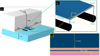 |
Fig. 1 a) Wind tunnel (shown only half) and the water domain of the model. b) FPV system, showing the frame and floating structure dimensions. c) The PV module’s layers. |
3.2 Air and water domains
The air mass flowing over the FPV system is infinitely large in real life. It is impossible to represent such an air mass for modeling purposes. As a result, it's critical to create a limited air domain surrounding the FPV system that's as tiny as feasible while nevertheless simulating the limitless air mass found in real life. To generate the air domain, Franke et al. [66] COST recommendations for CFD modeling in an urban context are used. The recommendations suggest utilizing a cuboid volume whose dimensions are determined by the characteristic height Hb, which is the highest obstacle's height. The top, sides, and inflow boundaries of the computational domain should be at least 5 Hb away [66]. A value of 10Hb is necessary for the outflow boundaries to ensure the influence of the target building is negligible [67]. Stated differently, the region behind the built area should be far enough away from the wake region to allow for flow redevelopment. The water dimensions in upstream, downstream, and lateral directions are set the same as the air domain. The water areas where FPV systems are installed tend to be shallow (1-4 m) [32]. Therefore, the water depth is chosen as 1 m to reduce computational time. This constitutes the geometry of the reference FPV system, and it is illustrated in Figure 1, Figure 1 along with the dimensions used.
3.3 Multiphysics settings
Aluminum is used for both the frame and the supporting attachments extending out of the frame. HDPE is used for the floating structure. The physical characteristics of the various materials are used to determine thermal resistances and capacitances. When an absolute value for the material property could not be obtained, the average between the values reported in the literature was taken instead. Table 2 lists the thermal properties of the materials used in the model. For radiative heat transfer, The emissivity of a substance is a measurement of how effectively it radiates heat. The emittance of PV glass and the back sheet is set to 0.9 [68].
Computational fluid dynamics was used to study wind flow over PV modules. CFD can resolve the RANS equations. Furthermore, by utilizing a verified CFD model, it is feasible to predict and enhance the thermal performance of a particular PV module design, considerably decreasing the time and money spent on testing. It is important to solve the viscous sublayer for accurate temperature profiling. The standard k—ω and SST k ω− models can resolve such layer, but they differ in one aspect. A reverse pressure gradient arises when the fluid contacts a sharp edge, such as a module, and the fluid is reversed. Menter's [69] SST−k ω model correctly predicts unfavorable pressure gradients and separation compared to Wilcox's [83] conventional k—ω model. Shademan et al. [70] demonstrated how the SST model performed well for flow around an inclined plate. This makes SST the model of choice employed in this paper. In a FPV environment, the air density will change with temperature. Thus, the air is approximated as weakly compressible, indicating that density is a function of just the temperature and does not vary with pressure. Furthermore, the gravity force is accounted for in this model.
The ground and every solid wall must have a no-slip boundary condition, with no slip meaning zero normal velocity. The lateral sides and top domain boundaries are treated as slip walls. An inlet wall with a boundary condition of velocity was chosen. At the outlet, zero gauge pressure is specified. A wet surface node for the modeling of evaporation and condensation was employed as well. Lastly, the symmetry plane cuts down the geometry to one-half and accelerates simulations. The simulations omitted two kinds of physics that occur in real life. The first is water movement and wave characteristics physics. Most FPV systems are installed in calm waters (lakes, lagoons, reservoirs, rivers, canals, etc.). Second, the solar radiation will be modeled as a heat source inside the module. The value of which is decided in the next section.
In this paper, we assumed the PV module's efficiency as constant at 18.4%. Also, the cell absorbs only some of the irradiance falling on the panel. Nizetic et al. [71] used an absorption coefficient of 0.86, which is used in this paper as well. Combining the last two values, this model converts approximately 70% of the irradiance into heat. Empirical (regression-based) or deterministic (physical-based) models can be used to forecast and measure water temperature. Empirical models rely on statistical regression to create less sophisticated models. Harvey et al. [72] suggest an equation that makes use of ambient temperature (Ta) to deduce a value for water temperature (Tw). However, placing water temperate under user control will be easier to better isolate the impact of water temperature alone quantitatively. Thus the water temperature will be independent of the ambient temperature in this paper. The water was set at 3 °C cooler than the ambient in the reference scenario. Table 3 summarizes the default geometry-based values and the physics-based ones used in the paper.
The angle of attack α signifies the wind direction and a value of 0° indicates the wind's first impact is on the tilted front surface of the module. The default wind velocity of 4 m/s is chosen as the median wind speed in Belgium. The same goes for the irradiance of 600 W/m2. The diffusion coefficient of water into the air at 25 °C is around 2.6 m2/s [73], and the evaporation rate is kept at its COMSOL default of 100 m/s. The RH was set at a neutral start of 50%. For a steady-state problem, the quantities do not change with time. Stationary simulations indicate that all quantities have reached equilibrium. The heat flux exchanged media via conduction, convection, and radiation processes balance the heat created within. For both steady-state and transient simulations, Nizetic et al. [71] proved that the converged panel temperature remained unchanged, allowing for a steady-state analysis, which is the case employed in the paper.
The thermal properties of the materials used throughout the paper (∗ Indicates values obtained from COMSOL material library).
The reference parameter values used in the simulations.
3.4 Mesh creation and grid independency test
Because a domain has an unlimited number of points, there are an endless number of equations to solve. The computing domain is discretized to a finite number of elements N to address this problem. For 3D geometries, the mesh generator discretizes the domains into a tetrahedron, hexahedron with a quadrilateral base, prism with a triangular base, or pyramid mesh elements.
The geometry is partitioned into multiple subdomains to facilitate the meshing. An inner air box of dimensions Hb is created inside the larger wind tunnel, which surrounds the FPV system. Because a combination of hexahedron and tetrahedron cells offers better results than a strict tetrahedron grid, the inner air block is used to decrease the number of tetrahedron meshes as much as feasible [66]. Arrangements of the elements are: hexahedron cells on the surface interior of the FPV system, tetrahedron cells in the interior air block encompassing the FPV system, then hexahedrons again for the remainder of the large air tunnel. The model is meshed using the "swept mesh" structured mesh type. Sweeping a source face to an opposing destination face is how the swept mesh works, and in the sweep direction, a swept mesh is built.
For solar modules, the velocity field changes quite rapidly in the normal direction. This observation motivates the use of a boundary layer mesh, a unique meshing approach. A mesh with dense element distribution in the normal direction along certain boundaries is known as a boundary layer mesh [74]. To make a boundary layer mesh, three values are needed. First, the height of the first layer of cells. Through trial and error, it was found that a value of 0.08 mm was adequate. Smaller values take longer to converge without large deviation in outcomes. On the other hand, larger values do affect the solution and are considered an example of under-meshing. Second, the boundary layer stretching factor is used to express the thickness increase between two successive layers; for example, entering 1.3 indicates a 30% increase in thickness from one layer to the next. Third is the number of boundary layers. It was decided to link the last two values together to obtain a boundary layer with total thickness of 10 mm. Hence, a stretching factor of 1.27 with 15 boundary layers was used. Figure 2 demonstrates the created mesh.
It can be seen in Figure 2b that the unstructured tetrahedron mesh shares an interaction with the topmost layer of the stack of boundary layer components, and the connection is made through a pyramid element. More importantly, the created mesh obtains a y+ < 1 on all the module's surfaces, shown in Figures 2c and 2d, indicating the turbulent boundary layer, including the viscous sub-layer area, is resolved to the panel surface. Thus the application of wall functions, which overestimates the convective heat transfer by 60% [75], is eliminated.
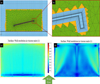 |
Fig. 2 a) Elements used to construct mesh, blue = hexahedrons, orange = pyramids and green = tetrahedrons. b) Zoom in demonstrating boundary layer meshing. c) and d) Results of y+ on top and bottom module faces respectively. |
3.5 Finite element model grid independence test
COMSOL uses the finite element method (FEM) to compute simulations. When using FEM, the accuracy of the solution is linked to the mesh size. As mesh size decreases towards zero, solutions tend to be the exact solution. However, an approximation of the solution will suffice due to limited computational resources and time. A grid convergence index (GCI) analysis, which estimates grid uncertainty and is derived from the generalized Richardson extrapolation, is used to report uncertainty owing to discretization in CFD applications [76]. It involves comparisons of discrete solutions at different grid spacings. A GCI study has two primary purposes: to establish convergence and to determine the rate of convergence p. To check grid independence, a set of five meshes with a different number of elements were created. Namely, the meshes are ranked from coarsest to finest based on the number of elements. G5 with 150 · 103, G3 with 374 · 103 and G1 with 853 · 103 elements. The grids contain these specific number of elements such that the grid refinement ratio r between grids is set to 1.3 in accordance with Roache's guidelines [76]. First-order discretization schemes are used for all unknowns: pressure, velocity, temperature, and humidity of their respective governing equations. Table 4 confirms that the solution does not change by monitoring the temperature, velocity, and pressure. This indicates that the numerical simulation's reliance on the grid has been lessened.
For a grid refinement ratio of r = 1.3 and the first order of the used numerical method, the GCI should be around 10% or less, as reported by Roache [76] which is achieved as reported in Table 4. Another metric of convergence is that the results approach the extrapolated solution f0. The apparent order of accuracy ‘p’ and the corresponding GCI xy matches with what was reported in literature [76,77]. Moreover, the consistency of the computed apparent order with the formal order is a good indicator that the grids are in the asymptotic range. From the table it can be seen that for the tested cases, asymptotic range where GCI36/(r13p.GCI13) ≈1 is ensured [76]. Another way of proving mesh convergence is through temperature, velocity, and pressure plots across the different grids. The mesh convergence plots are shown in Figure 3. Based on the previous, the average grid G3 and fine grid G1 gave almost co-incident results, indicating mesh convergence. Given the computing resources available, G3 is chosen as the final grid for simulation.
GCI computation across three grids for different physical quantities. Temperature measurements are averages.
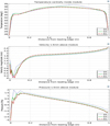 |
Fig. 3 Plots of temperature, velocity and pressure from left to right respectively. |
3.6 Model validation with experimental results from the literature
The simulation work of Nizetic et al. [71] was replicated; if both results were close to each other, then the model was verified. First, their simulation was for a standard GPV system. Hence the water domain was removed. Then the same settings of wind speed and irradiance were applied. Their results showed that the average temperature for G = 800 W/m2 and U = 3 m/s was 43 °C. In the constructed model, the average temperature reading was 44.8 °C. A relative error value of 4%. The most probable explanation is that in the Nizetic simulation, the module was assumed to have an efficiency of 19.5%, while in this paper, the efficiency was considered to be 18.4%. Lower efficiency indicates a larger heat source and, thus, a larger temperature reading. Nonetheless, the model was validated to be accurate enough to proceed.
4 Results and discussion
After each simulation, the results are post-processed and analyzed to minimize ambiguity and maximize understanding. Whenever possible, the results obtained are compared with literature results, whether they agree or disagree. Lastly, a conclusion is made regarding which theory is the most probable for FPV cooling.
4.1 Comparing FPV with GPV
The first simulation compares FPVs against GPVs since that seems to be the industry standard. It must be noted that the systems were simulated in the exact same environment. The default parameters listed in Table 3 were used for both simulations. Meaning, both systems experience the same wind speed, RH, ambient temperature, etc. The only difference is that water is swapped out for soil when simulating for GPVs. This essentially states that the only differentiating factor between the FPV and GPV simulations is the existence of water. With that being said, the simulated module temperature in both scenarios came out to be identical at 34.71 °C. This is obviously the exact opposite of what was expected which was a minor or major cooling for the FPV module. Concluding that water has proved ineffective in cooling but further analysis is needed to know why.
Figure 4 shows how water changes the surrounding air. What is shown is the portion of air directly underneath the module. It is demonstrated in Figure 4a that at the water surface (altitude = 0 mm), the air is completely saturated with water vapor molecules. This is clearly indicated by having air at 100% RH. It can be described as water-like air and this translates into air temperature as well as shown in Figure 4b. The water temperature was set to 22 °C and the air directly at the water level has the same temperature reading. Up till now, the theory of evaporative cooling is working just as intended. The water is providing an extremely valuable benefit of cooling the surrounding air. Unfortunately, this cooling effect hardly continues any further away from the water level. Once only 5 mm away from the water, the water properties that were given to the air dramatically dissipate to the environment. The air no longer becomes saturated with water vapor, and, consequently, has a temperature that is much higher than water temperature. The further away the air is from the water, the less water-like the air becomes. At an altitude of just a mere 1 cm, the air that used to carry some water properties has now become very similar to ambient air. At around 5 cm and beyond, the air becomes indistinguishable from the ambient air already present. Meaning the portion of air actually nearby the FPV system has a RH of 50% and a temperature of 25 °C. Both of these are the exact same settings used in the GPV simulation, making the air around the FPV module identical to the one surrounding the GPV module. This explains why both FPV and GPV modules had the same temperature.
In short, while evaporative cooling of air is proven to take effect for FPV systems, the effect is extremely lackluster and is only clearly present in the first cm away from the water. The evaporative cooling process changes air properties for the better but only at a small domain that will be termed a ‘Vapor Blanket’. This vapor blanket is a maximum 2 cm thick, and all air above said blanket retains very little to no features of the water body. Stated differently, the water is unable to induce a change that can reach the module level. So it can be said that the mere existence of water is not enough to induce any cooling to the panel. With all other parameters being equal, placing a PV system on top of water or soil will have no difference in operating temperature. In conclusion, the cooling process for FPVs is in need of a stimulus that does not originate from water. Thus more simulations are needed to see which parameter is most prominent for FPV temperature.
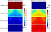 |
Fig. 4 Plots of a) Relative Humidity and b) Air temperature directly underneath the module at various altitudes from water level. |
4.2 Relative humidity impact
Since RH is one of the key components of the evaporative cooling process [78], in the sense that evaporative cooling efficiency is inversely proportional to RH level. One could expect that the lower the ambient RH level, the larger the vapor blanket will become. This is explained by the psychometric fact that humid air is lighter than dry. So the larger the disparity in RH levels, between the ambient air and the cooler air entrapped inside the blanket, the larger the blanket should be, ideally reaching the module and cooling it. A number of simulations were run with all parameters fixed except the ambient RH which varied from 0% to 100%.
As per the theory, the higher the humidity, the less dense the air became. This is clear in Figure 5. When the air is free of water vapor and completely dry, the density was around 1.184 kg/m3. On the opposing end when the air is saturated with vapor and humidity, the density dropped to nearly 1.171 kg/m3. A relative density drop of around 1%. More interestingly, the density change is more apparent inside the blanket. Once the blanket has expired, the remaining portion of the air still maintains the density of the air that was inside the blanket. In other terms, the air inside the blanket changes the density of the ambient air and not vice versa like in the previous section where the ambient changed the RH levels of the air inside the blanket. What remains to be seen however is if this density disparity had an effect on air temperature and consequently FPV temperature. Figure 6 holds the answer.
On the upside, when the ambient is dry, this gives more room for the blanket to rise since now there is a bigger density disparity. This can be better seen in Figure 6b. At a given altitude from the water depicted on the y-axis, the blanket is holding slightly cooler air if the ambient was dry. As the cooler air gradually rises, it can be stated that the effective thickness of the blanket has increased slightly or that the blanket remains the same thickness but is holding colder air, increasing efficacy. Also as expected, the higher the humidity, the worse the evaporative cooling operation performs. Because now both the ambient air and the air inside the blanket have similar humidity levels. This essentially acts as a barrier for the cold air inside the blanket to rise upwards towards the module. Hence, the blanket is now characterized by an even smaller effective thickness. The changes that RH prompts in air density and temperature are in line with expectations. On the downside, however, the density difference is not significant enough to induce large cooling. When the ambient was dry with 0% RH −which is the ideal scenario for the evaporative cooling process-, the module's temperature was 34.7 °C. Just 0.01 °C lower than the reference case with 50% RH. On the other hand, when the ambient is saturated with 100% RH, the module's reading was 34.72 °C. Symmetrically the opposite result, where here a heating of 0.01 °C is noted. The results obtained agree with the literature. Choi et al. [93] showed that the module temperature increases with humidity. A decrement of the air's RH is always desired as RH shortens module lifespan and has an impact on PV power output in a similar way to dust collection. Increased water content in the air increases solar radiation scattering and lowers solar intensity received. As a result, the solar cell suffers a loss in incoming energy.
In any case, these outcomes essentially refute the potential of evaporative cooling entirely. Simply put, the first theory of evaporative cooling is way too constrictive and does not stimulate a cooling that is large enough to match or even come close to the lower end of the cooling numbers reported in the literature of around 1–2 °C.
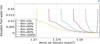 |
Fig. 5 Plots of air density at different humidity levels. |
 |
Fig. 6 a) Air temperature at different humidity levels. b) Close up plot. |
4.3 Ambient temperature impact
Ambient temperature is without a doubt one of the most important elements influencing PV module operating temperature (Tmod). Because heat convection is dependent upon the temperature differential between the surface and the air itself. The warmer the air is, the less heat is transferred from the module to the ambient air resulting in a warmer module. The opposite effect shall occur as the ambient becomes cooler, carrying more heat out of the module resulting in a lower temperature. The results of the simulations are written in Table 5 and they follow expectations.
When the ambient is cool (20 °C), there exists a larger temperature difference between PV and ambient, this facilitates heat transfer. The temperature differential between the module and the ambient reduces as the ambient temperature rises, reducing the rate of heat loss from the module to the environment [79]. Additionally, the relationship between ambient and FPV temperature is of linear nature, with a change of 0.85 °C for every 1 °C change in ambient.
No difference was found in the temperature distribution along the module. The hottest spot was always in the middle, especially downwind. The coolest spots were near the frame and at the upwind edge. In conclusion, the findings show that a lower ambient temperature aids heat dissipation and, as a result, improves the electrical efficiency of FPV modules like the findings of Kamuyu et al. and Zhou et al. [24,80].
This subsection validates the second theory in justifying FPV cooling since the simulations show that the ambient environment affects FPV temperature by a significant margin. However, to know with certainty whether the second theory is the sole, or partial, contributor to FPV cooling requires further investigations carried out in the following sections.
Change in module temperature with ambient temperature setting. Bold is the reference.
4.4 Wind speed impact
The third theory of FPV cooling was through wind velocity enhancement. Lower wind speeds result in less turbulence and hence, less evacuation of heat. Most literature agrees that module temperature changes linearly with wind speed [81]. However, the obtained results deviate slightly from this norm as shown in Figure 7. The obtained curve for module cooling shows a square-root dependency on the wind velocity, the same as the findings of Goverde et al. [4]. When wind speed is low (≤2 m/s), natural convection dominates, this results in a large jump in module temperature. As the wind speed increases, more heat is extracted from the panel, decreasing its temperature. This is attributed to the more turbulent nature of the airflow which improves heat transfer as compared to laminar flows [4]. Nevertheless, the cooling rate slows down as wind speed gets larger similar to the findings of Zhou et al. [80]. More than likely due to the better cooling performance which shrinks the temperature difference leading to smaller cooling for every 1 m/s increment in wind speed. Hence it can be concluded that FPV temperature is sensitive to wind speed, and more so at the lower end. It is a valid theory that higher wind speeds experienced by FPV systems will aid in cooling, leading to a better efficiency rating than GPVs. Yet, the parametric sweeps performed so far do not show the full picture yet. At this point, it is inconclusive to say which of the two theories, ambient temperature or wind speed, is the one responsible for FPV cooling. For these reasons, the following sections explore every other aspect regarding FPV operation. This will provide further understanding regarding the thermal workings of FPVs and a more decisive conclusion.
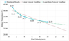 |
Fig. 7 Module operating temperature versus wind velocity. Dotted lines are linear and logarithmic forecasts. |
4.5 Water temperature impact
One key feature of FPV is water presence. It has already been explored that the positive effects of water on the surrounding air disappear quickly into the environment. This section investigates how the temperature of the water changes the vapor blanket and how major are these changes in the blanket to the module temperature. In order to keep the simulations compatible with real-life environments, the maximum difference between water temperature and ambient temperature was set ± to 5 °C [82]. This determines the water temperature span for this section's simulations.
The simulation outcomes show a significant correlation between water and module temperature. While the correlation is significant, the resulting cooling or heating is not. When the water temperature is at 20 °C, the module cools down to 34.46 °C, 0.25 °C lower than the reference. When the water temperature is set to 30 °C, the module heats up to just 35.7 °C, 0.99 °C warmer than the reference case. So there is a definite correlation but with small changes. A valid estimate is that the average FPV module temperature changes by 0.125 °C for every °C change in water temperature.
The reason for the correlation is the direct impact of water temperature on the air temperature inside the vapor blanket. This is demonstrated in the bottom portion of Figure 8. This creates a more favorable temperature gradient that cools down the module the colder the water is. The opposite effect is true the hotter the water. This explains why module temperature changes but the reason why the change is small is better demonstrated using the top portion of Figure 8. Where it becomes clear that regardless of water temperature, the air temperature will converge close to the ambient temperature (25 °C). Once the vapor blanket blends with the environment (occurs around 1 cm away from water), there is an extremely small difference in the temperature of the air that reaches the FPV panel, hence the small change.
Conclusively, the water temperature does indeed impact FPV temperature both positively and negatively. This is a key consideration as that would indicate worse performance for FPVs in the winter as during winters, the water becomes warmer than ambient. This observation was also evident in the work of Golroodbari and Sark [15]. The outcomes of the paper's simulations disagree with Hwang et al. [83] and Peters and Nobre [25] which state water temperature has no impact on FPVs. The outcomes agree more with Jeong's et al. study [26] with a moderately strong correlation between water and module temperatures.
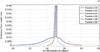 |
Fig. 8 Evolution of air temperature with elevation from water for different water body temperatures. |
4.6 Tilt angle impact
The tilt angle of panels that corresponds to local latitude is better for increasing annual power generation. Low tilt angles, on the other hand, are favored in FPVs [50,56] because they allow for a smaller space between rows, allowing for more area to be used and a reduction of wind forces on the structure. Furthermore, it was found that the flatter the panel, the less water was evaporated due to the reduction of water exposure to solar radiation. Since the common practise is low tilt angles, the simulations span from θ = 0° till 50°, in increments of 10. Higher tilt angles were not encountered in practise nor in literature experimentation.
The results of the simulations were as follows, for a flat panel, the average temperature was 34.75 °C. Slightly higher than the reference (θ = 10°) which sat at 34.71 °C. As the angle increased to 20° and 30°, so did the temperature, reaching 34.95 °C and 35 °C respectively. But with a further increase in tilt, the opposite observation is noted. For the angles of 40° and 50°, the module temperature reduced to 34.8 °C and 34.7 °C. To better explain this unsteady trend, a closer look into wind behaviour is required. Figure 9 illustrates the wind streamlines for the simulated tilts.
Three phenomenons occur to the wind profile. The first, is flow detachment (green box in θ = 0° in Fig. 9). This occurs as the wind strikes the leading edge of the module. The detachment divides the wind flow into two parts, the major part will go and glide over the front side of the module all the way to the trailing end, the second part will flow down and around the aluminum frame and converge with the streamlines coming from the inlet. The second phenomena is the recirculation bubbles/zones (pink box in θ = 20° in Fig. 9). Close to obstructions, the wind deviates from its normal course, resulting in intricate recirculating patterns known as vortices. Winds spread outwards away from high high pressure to low pressure places. Since the entire backside of the module sits at low pressure, the wind will aim to go towards this low-pressure region instead of continuing towards the outlet. This leads to the third phenomena which is return flow (red box in θ = 40° Fig. 9). This is more prevalent in higher tilt angles as now the pressure imbalance becomes larger, this will encourage more wind to flow back towards the backside of the module. The flat panel heated up because the inclination makes it that less panel area is impacted by wind, the flow detaches and then reattaches at a much later point because of the lack of any inclination. By increasing the tilt, more panel area is coming into contact with the wind. So one expects better cooling with an increment of the tilt angle which is true for θ = 10° but not for larger angles. As tilt angle increases, both the vortex and return flow get larger. But for the case of 20° and 30∘, the module experienced a heating because the return flow was not as strong as the one for the 40° and 50° tilts. The latter two cases experience a higher wind speed contact at their back side resulting in lower temperature than in the earlier two cases of 20° and 30°.
To conclude, the paper outcomes would disagree with the literature which supports the general finding of better convection with increments in tilt angle [84–86]. The finding of the paper are more case specific but they prove that the low tilt angles common for FPVs will not hinder performance by a large degree. The optimum angle was found to be 10° like the findings of Ueda's et al. [87] FPV project where the angle was changed from 1.3° to 10° to enhance air cooling.
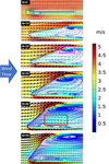 |
Fig. 9 Streamlines of wind velocity for different module tilt angles. |
4.7 Wind direction impact
So far the module was placed such that the incident wind's first point of impact was on the front side of the panel. Indicating that wind was perpendicular on the module's front surface. Wind direction is often characterised by the angle of attack α. The default has been 0° so far. This section sweeps over the possible directions where wind can originate from. The results of the simulations are illustrated in Figure 10. It can be noted that in all scenarios, the coldest region of the module is also the region that is closest to the wind inlet. On the other hand the hottest spots are at the opposite end of the panel, at the downwind located regions. This is best shown for the case of α = 90 °. This phenomenon is explained by the air's boundary layer. At initial impact, the wind is at ambient temperature and is characterised by high velocity. Both of these characteristics provide a cold spot at the leading edge. Further down, the wind separates and then reattaches at a later point. A boundary layer forms after reattachment. This barrier layer stores heat [88], resulting in a reduction in heat transport. Hence why temperature of the downwind-located portion is highest [3].
Moving from hot and cold spots to averages, one notices the following trend plotted in Figure 11 for not only the default θ = 10° but for a flat panel and a pane tilted 20°. As α increases, the heat transfer rate decreases similar to the outcomes of Turgut and Oner [89] and Wu et al. [90]. The effect persists till and including α = 90° which carries the highest module temperature. With further increase of α, we return back to oblique winds (α = 45° and α = 135°) which are characterised by a higher temperature than the reference case of α = 0°. Lastly, the scenario when the wind makes first contact with the back-side of the module showed a higher temperature than the oblique winds even though more panel area is in contact with the inlet wind. This is attributed to the unfavorable inclination and the aluminum frame both of which make the flow separation more severe. The previous explanation also applies to the other two tilt angles tested. One note to make is that the flat panel is the least sensitive to deviations in α. It still conforms to the bell shape but to a lesser extent as θ = 10° or 20°.
To sum, the convection by wind is at its maximum when the wind is falling perpendicularly on the panel. Moreover, this section demonstrates that wind direction has a considerable impact of the operating temperature of FPVs. The fact that manipulating wind direction alone had a more significant impact on FPV temperature compared to water temperature, is already an indication that the third theory which supports cooling of FPVs due to convection is definite contender to justify better FPV performance. However, even more analysis is still needed which follows next.
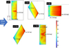 |
Fig. 10 Top view of FPV temperature profiles for various values of the wind direction (α). |
 |
Fig. 11 Temperatures simulated for different wind directions. |
4.8 Solar irradiance impact
The amount of radiation absorbed by the module largely dictates its temperature. The irradiance intensity is by far one of the most impactful parameters. As a reminder, the user inputs the solar irradiance (G) and not the heat source (Q). The heat source is what is left from the irradiance after factoring in the efficiency and the absorption coefficients for the different layers. Table 6 documents the consequences of the simulations.
As expected, by increasing heat flux, the operational temperature of PV panel increases. It is observed that the module temperature is linearly proportional to irradiance like in [91]. The change in FPV temperature is around 1.6 °C for every 100 W/m2 change in irradiance. The temperature patterns and distributions for the reference irradiance case are shown in Figure 12a.
The temperature distribution throughout the surface of the module reaches its highest in the middle and its lowest near the edge, a similar pattern as the results by Zhou et al. [80]. With a specific notice that the downwind zone is slightly hotter due to heat entrapment in the boundary layer. To see where exactly on the module will a change in irradiance change the temperature, Figures 12b and 12c show the cases for cooling and heating. In the cooling case, the irradiance is dropped from the default 600 W/m2 to 200 W/m2. The area that experienced the largest cooling was down the center. A similar observation is noted for the heating case when the irradiance increased from the default to 1000 W/m2. Majority of the acquired heat was concentrated down the middle. This is because the underlying heat transfer method remains the same. In other words, both convection and conduction are still present and contributing. However, their contributions are low during low irradiance, as the module's temperature approaches ambient. The opposite is true where high solar irradiance helps dissipate heat out of the module because of the larger temperature difference between PV and ambient. However, the increased solar irradiation results in a larger input energy than the heat transported out, resulting in a higher panel temperature [80].
Average panel temperature for different amounts of irradiance. Bold indicates reference FPV settings.
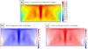 |
Fig. 12 Wind flow from bottom to top. a) Temperature contours for the reference panel. b) Temperature difference between Q = 200 W/m2 and Q = 600 W/m2. c) Temperature difference between Q = 1000 W/m2 and Q = 600 W/m2. |
4.9 Water proximity impact
By now it is an established fact that near the water surface, the air becomes cooler since it picks up water vapor and gains some of the water's characteristics. This was especially evident in the vapor blanket where the air characteristic dramatically change to become similar to that of the water's. Thus one would logically assume that installing the FPV module closer to the water shall yield a benefit in cooling. Simply, since the module is now closer to a cold surface, the operating temperature should decrease as well. This section investigates how FPVs are affected by the clearing distance left between the bottom edge of the aluminum frame and the water surface. The simulation results are presented in Figure 13.
Quite the opposite to expectations, the closer the module was placed to the water, the warmer it became. This is by far the most debatable result obtained across all parametric sweeps. Vega Orrego [47], Desai et al. [92], Rodrigues et al. [93] and Hayibo et al. [94] all state better cooling and performance the closer the modules' are placed to water, as then the modules' take better advantage of water cooling. Despite all this evidence supporting better cooling with closer water proximity, the opposite effect found in this paper is perfectly explainable.
Velocity magnitude changes with elevation in the sense that the closer the module is to the water, the lower the wind velocity striking the module. The further away the system is from the water, the higher the exposure of the panel to the open air and hence, the lower the temperature. This all goes back to how wind interacts with walls. In this case, the wall (water), is reducing wind speed due to friction. The reduction in velocity is outweighed by any other benefit that the FPV enjoys, for example, a cooler surrounding environment coming from the vapor blanket. The temperature and wind velocity plots that show such an effect for the FPV at three elevation scenarios are shown in Figure 14. Another observation noted in both Figures 13 and 14 is that the FPV temperature increased slightly with an increment of the clearing distance above the default of 20 cm. This can no longer be attributed to a change in wind velocity since at such a large clearing, the wall (water) has no influence on velocity. The larger clearing allows the air coming out of the blanket more distance for recovery. During this recovery distance, the air will start to revert back to its ambient character. Slowly gaining temperature till equalisation with ambient air. By the time the air reaches the module, the surrounding environment is no longer cooler than ambient. This is the more than likely explanation why placing the module further than 20 cm away results in a slightly higher operating temperature.
To sum, there exists a specific distance away from the water where the FPV will benefit from both the fully developed wind flow and the temperature gradient from the blanket that creates a cooler environment. This is an optimization problem by nature that is out of the scope of the paper but from the results, it seemed that the default of 20 cm was most optimal to benefit from both water and wind. In any case, close FPV proximity to water is ill-advised in practise, the high RH and chloride accelerate PID and corrosion [28].
The results are another piece of strong evidence that FPV cooling is through wind. FPVs are highly dependent on good air ventilation. The experimental work of Liu et al. [22] indicated due to efficient air circulation, the free-standing kind offers great cooling efficacy. Cooling was reduced in the other variants, which had modules located close to water. When module is very close to water, wind has smaller role and water has larger role. Since a warming of the module was noted, it would highly encourage the theory of convective FPV cooling, and that water serves minor influence.
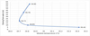 |
Fig. 13 FPV temperature vs clearing distance. |
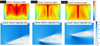 |
Fig. 14 Temperature distributions and wind flow for three different clearings (height from the water level is changed) |
4.10 Evaporation rate impact
One of the parameter input of the simulations was the evaporation rate constant Kevap. It is an indication of how much water is being evaporated per unit time. From the outcomes of the paper so far, water has been lackluster in cooling the FPV module. It could be possible that evaporating more water in a shorter time span will make the blanket thicker leading to more heat extraction. However, due to the stationary nature of the performed simulations, seeing the effect of evaporating water on the air as time passes is not possible. Such a result would require a time-dependent simulation which is computationally too prohibitive. Regardless, a simulation set spanning a range of Kevap values was performed in a time-independent manner.
The simulations showed no effect on FPV temperature. This is because the simulations are in steady-state, where the end solution is displayed which is not affected by the evaporation rate. This corresponds to assuming that vapor is in equilibrium with the liquid. Hence, Kevap has no effect on end temperature or RH indices. In practice, it is expected that the quicker the rate of evaporation, the greater the cooling [78]. But even then, this is only applicable inside the vapor blanket, the remaining air domain remains indifferent and experiences little to no cooling.
4.11 Water depth
The water depth employed so far was 1 m. This value is not the most reflective of the water depth of real-life FPV installations which might be deployed in deeper waters. A positive correlation was obtained between deeper water and cooler modules. However, the significance is in the range of just 0.04 °C between 1 m and 6 m deep water. It is not known with certainty why shallow water would lower FPV temperature. Nothing was found in the literature that presents the same correlation. One possible explanation is the following. Water depth is found to have almost a one-to-one correlation with distance from the shore. In other words, the further offshore, the more likely that the water is deeper. It is also known that further offshore, wind speed is larger due to having fewer obstacles and enjoying a longer fetch. Deeper water can be associated with more open space to build up wind speed or less surface roughness to restrict wind speed. In either case this leads to an increase in wind speed near the module as shown in Figure 15. Whereas the deeper water scenario sees a slightly faster wind speed close to the module's leading edge. This would explain the lower operating temperature. Further experimentation is needed to confirm the positive minor correlation between water depth and FPV performance.
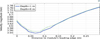 |
Fig. 15 Approaching wind velocity for 1 m and 6 m deep waters. Movement to the left on x-axis means approaching module. |
4.12 Power plant characteristics
Just like their GPV counterparts, FPVs are built on large scales as power plants supplying MWs of power. Hence, from both an engineering and economic standpoint, one desire to know which power plant configuration will lead to the lowest average PV temperatures and hence the best power output and return on investment. There are four possible combinations encountered in practice, they are shown in Figure 16. The simulations will still maintain the default parameter values listed in Table 3. The distance between the two panels is set to a fixed value of 60 cm. For simplicity, the panel closest to the inlet is given the name ‘P1’, and the other is named ‘P2’. Furthermore, the configurations will be given a letter instead of a description similar to as displayed in Figure 16. The temperature outcomes of simulating the four installations are shown in Figure 17. The PV panel's average temperature was calculated by summing up all the PV surface temperature nodes and dividing by the number of nodes. It can be seen that configuration ‘A’ shows a similar average temperature for both panels. In configuration ‘B’, both panels experience fair heating. While in installations ‘C’ and ‘D’, only ‘P1’ sees remarkable heating while an opposite effect is observed for ‘P2’ which cools down marginally. The results are best explained through observations of the wind and temperature profiles illustrated in Figure 18.
For configuration A, P1 sees the incoming developed wind and hence cools down as expected. Conversely, P2 sees slightly weaker wind flow due to the blockage of P1, hence heating P2 up slightly. For configuration B, one would assume that P1 would have the same temperature as P1 in configuration A since they both experience the same wind and orientation. Instead, P1 heats up to 34.95 °C, this is explained by the lack of wind on the back side of P1. In configuration A, the recirculating wind successfully flows to the back side of P1 while in configuration B, the wind is unable to flow back towards P1 because of the orientation of P2. Admittedly, P2 acts as a wall that prevents P1 from cooling down further. It is worth to note that an increase in the spacing between the panels will likely fix such an issue. Unfortunately, simulations varying the spacing could not be performed due to time constraints. Further, the larger the spacing, the more costly the power plant commissioning will be. More than likely, the advantage of operating the modules at slightly lower temperatures will not compensate for the additional financing needed for the added water area. P2 in configuration B sees large heating because of its inclination and orientation both opposing the wind inlet. Hence experiencing poor wind flow. P1 in both configurations C and D had the largest recorded temperature. The explanation for both is the same, the orientation of P1 doesn't allow its front side to get any cooling whatsoever. The flow detaches at the leading edge but it does not circulate back to P1. Yet it continues onward toward P2. Couple with that the strong wind coming from the ground level because of streamlined convergence. Both of the previous observations allow P2 to be cooled significantly. The streamline convergence is more apparent in configuration D than C, this is why P2 shows a lower temperature at the bottom portion for installation D.
One key point that has to be made here is the following. Those supporting FPV cooling through water or ambient temperature would have a valid argument if and only if both panels in any configuration showed similar temperature readings. For the reason that both water and ambient temperature are not spatially variant in the simulation environment while the air is. Unquestionably their effects would be felt by all panels in all configurations in generally speaking equal magnitude. The difference in temperatures between P1 and P2 across all installations signifies undoubtedly the importance of wind in the thermal operation of FPV plants.
 |
Fig. 16 The four studied power plan tconfigurations. a) Both modules facing wind inlet. |
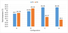 |
Fig. 17 Average PV temperature per panel for the four power plant installation types. |
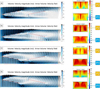 |
Fig. 18 Wind and temperature profiles for all configurations. Modules and frame are colored red for clarity. In the velocity temperature plots, P1 is on the left. |
5 Summary of the finite element modeling results
This section will nail down why exactly are FPVs reported to be cooler than GPVs. The simulation sets performed earlier can be split into two categories; one is water-related parameters, and the other is ambient or wind-related parameters. For the earlier, the simulations included studying RH, water temperature, evaporation rate, diffusion coefficient, and water depth. The latter group included studying ambient temperature, wind speed, tilt angle, wind direction, solar irradiance, turbulence intensity, and power plant behavior. The water-related parameters exhibited minimal to insignificant variations in response to the FPV temperature. In contrast, the ambient or wind-related parameters displayed minor to noteworthy influences on the FPV temperature. Based on the aforementioned observations, it can be inferred that water has a limited to negligible contribution to the performance of FPV modules.
The visual aspect may be the primary reason why individuals commonly associate water with the cooling of FPV panels. On an eye-to-eye basis between a low-efficiency GPV and a higher-efficiency FPV, people are quick to point out the key difference: the existence of water. Hence they associate high efficiency with water. However, this study presents a different finding. It establishes that whenever the FPV outperforms the GPV, the improved performance can be attributed to one of the following factors: either a decrease in ambient temperature (referred to as Theory 2) or an increase in wind speed (referred to as Theory 3) as stated in this paper.
Since both theories 2 and 3 hold the most truth when it comes to claiming FPV cooling, a demand to know the sole reason for cooling exists. To isolate which is more dominant, a sensitivity analysis was performed and compared to the reference FPV system. This will help see the deviation in module temperature against a 1–2 m/s wind speed difference or against a 1–2 °C ambient temperature difference. The temperature difference is then converted to expected efficiency gain from the use of the heat coefficient value of 0.0045 %/°C. The outcomes of the sensitivity study are presented in Table 7. It turns out that a 1 or even a 2 unit change in ambient temperature is less impactful to the module compared to wind speed. In other words, for a step size of 1 or 2 units, wind dominates ambient temperature when it comes to affecting FPV temperature. Therefore, it is evident that wind speed bears greater significance in cooling the FPV module. Furthermore, if ambient temperature conditions were solely responsible for FPV cooling, it would be expected that the literature would consistently report poorer FPV performance during winter seasons. However, such observations are rarely encountered, indicating that ambient temperature is less likely to be the primary factor in FPV cooling. Considering the evidence presented thus far, this paper concludes that the improved cooling of FPVs can be attributed to the enhancement in wind speed.
As for the extremely high gains reported in the literature, the only possible explanation is a lack of understanding and over-advertising. The same flaws that encircle any new technology. Moreover, experimentation, where FPV is compared to another case, has to abide by a key rule; otherwise, you risk location bias. As a recommendation for future experiments, the FPV and the comparison case must be located as close to each other as possible. The further the distance, the more exogenous parameters take effect, which hinders the findings of an irrefutable conclusion. The simulated energy increase in output using FPV technologies is less than the literature's predicted values, which are equal to or greater than 10%. A more realistic, conservative and recently-supported-in-literature value is around 0.5–3% depending on the FPV environment's parameters.
Sensitivity analysis of ambient temperature and wind speed variations on FPV module temperature.
6 Conclusion
Along with the land savings of FPVs, came a belief that FPV modules have superior thermal performance than GPVs. The cooling claim was ill-understood and quantified. This paper was written to understand the thermal dynamics of FPVs. This cooling can be attributed to one of four theories. Evaporative cooling, ambient temperature, wind speed, and heat transfer by conduction. To decide upon the true reason behind FPV cooling, a simulation model was created. A number of parametric sweep simulations were performed to measure the impact of each parameter on the thermal workings of FPVs. The simulations' most important outcomes can be stated as follows:
Decreasing the RH of the ambient air increases the efficiency of the evaporative cooling process. But the improvement is minor in the range of 0.01 °C. Debunking the theory that FPVs can be cooled through water evaporation.
Ambient temperature heavily affects FPV temperature. The relation is linear with a difference of 0.85 °C per degree change in ambient temperature.
Wind velocity contributes to cooling the FPV module. However, the sensitivity of module temperature to wind speed is large at low speeds and decreases with increments in wind velocities. Presenting a non-linear relationship.
A correlation between water and FPV temperatures was found. Despite this, the quantity of the correlation is small. The module's temperature changes by 0.125 °C for every degree change in water temperature.
The tilt angle did not make a major difference in a single-array simulation. No large disadvantage of laying the panel flat or at a high tilt was found. The recommendation to keep FPVs at low tilt angles will not hinder FPV performance.
FPVs are sensitive to wind direction. Parallel winds show the largest cooling. Oblique wind and backward wind result in slight warming. The hottest module was obtained when the wind was 90∘ incident on the system.
Laying the FPV system closer to the water was found detrimental to performance. This is attributed to worse incoming wind flow. The wind near the water experiences more friction which slows it down. Placing FPVs away from the water allows for better ventilation.
Expanding the model to simulate power plant behavior for different configurations showed varying panel temperatures for all configurations. This stipulates the heavy dependency of FPV operational temperature on wind flow and the smaller dependency on water or ambient temperature.
The fourth theory of cooling through conduction is disproven based on three factors: the small temperature gradient, a limited contact area between the PV module and floating structure, and extremely low thermal conductivity values. These factors restrict heat transfer through conduction, resulting in a mere 0.5 °C temperature difference in FPVs.
Out of the two most probable explanations for FPV cooling, the sensitivity analysis showed higher reliance on wind speed than ambient temperature.
Ultimately, all evidence presented in the paper points towards the cooling of FPVs through higher wind speed on open water bodies. Generally, the findings show once more that one should be wary of generalizations. Further, while it is possible that FPVs have higher proficiencies, the expectations should be more conservative at a maximal 3% gain. Despite that, the outlook for FPV is positive and is set to break free of its niche status. For future work, the development of a model that accounts for different designs, power plant sizes, and energy calculations is needed. Further, more experimental work is encouraged to concur with the results obtained in this paper and the literature. A recommendation for future study is to experiment with FPV and GPV in the exact location to eliminate uncontrollable variables.
Abbreviation
CFD: Computational fluid dynamics
DNS: Direct numerical simulation
EVA: Ethyl-vinyl acetate
FF: Fill factor
FEM: Finite element method
FPV: Floating photovoltaic
GCI: Grid convergence index
GPV: Ground-mounted photovoltaic
HTC: Heat transfer coefficient
HDPE: High density polyethylene
LES: Large eddies simulation
NS: Navier-Stokes
PV: Photovoltaic
PVT: Photovoltaic/thermal
PID: Potential induced degradation
RH: Relative humidity
RANS: Reynolds averaged navier stokes
SST: Shear stress transport
TI: Turbulence intensity
WVC: Water veil cooling
Symbols
A: Module's surface area (m2)
c: Concentration (mol/m3)
Cp: Specific heat capacity at constant pressure (J/(kg · K))
D: Diffusion coefficient (m2/s)
F: Buoyancy force (N/m3)
f0: Extrapolated solution
G: Solar irradiance (W/m2)
gevap: Evaporation flux (kg/(m2·s))
Hb: Characteristic height (m)
I: Diode current (A)
IL: Photo-generated current (A)
Io: Reverse/Dark saturation current (A)
Isc: Short circuit current (A)
Kevap: Evaporation rate (m/s)
k: Turbulence kinetic energy (m2/s2)
K: Thermal conductivity (W/(m · K))
L: Length scale (m)
Lvap: Latent heat of vaporization (J/kg)
Mv: Molar mass (kg/mol)
Pmax: Maximum output power (W)
p: Absolute pressure (Pa)
P: Rate of convergence
Q: Heat source (W/m2)
qevap: Heat flux during evaporation or condensation (J/m2 · s)
R: Specific gas constant (J/(kg ∗ k))
Re: Reynolds number
r: Grid refinement ratio
T: Absolute temperature (∘C)
Ta: Ambient temperature (∘C)
Tmod: Module temperature (∘C)
U: Instantaneous velocity (m/s)
u: Velocity vector (m/s)
u+: Velocity vector in viscous units
uI: Fluctuation velocity (m/s)
uτ: Frictional velocity (m/s)
Voc: Open circuit voltage (V)
y: Distance to wall (m)
y+: Distance to wall in viscous units
z0: Aerodynamics roughness length (m)
Greek letters
α: Wind direction (∘)
αabs: Absorption coefficient
ε: Turbulent dissipation rate (m2/s3)
η: Conversion efficiency (%)
θ: Tilt angle (∘)
μ: Dynamic viscosity (Pa · s)
μT: Turbulent viscosity (Pa · s)
ν: Kinematic viscosity (m2/s)
ρ: density (kg/m3)
τw: Wall shear stress (Pa)
ϕ: Relative humidity level
ω: Specific dissipation rate (s−1)
Author contribution statement
Gofran Chowdhury: Conceptualisation, Methodology, Formal analysis, Visualisation, Writing – original draft. Mohamed Haggag: Formal analysis, Data curation, Visualisation, Writing – original draft. Jef Poortmans: Conceptualisation, Writing – review ∓ editing, Supervision, Funding acquisition.
References
- M.G. Chowdhury, A. Kladas, B. Herteleer, J. Cappelle, F. Catthoor, Sensitivity analysis of the state of the art silicon photovoltaic temperature estimation methods over different time resolution, in 2021 IEEE 48th Photovoltaic Specialists Conference (PVSC) (2021), pp. 1340–1343 [Google Scholar]
- G. Chowdhury et al., Novel computational fluid dynamics modeling of spatial convective heat transfer over PV-modules mounted on an inclined surface with an underlying air gap, in 35th European Photovoltaic Solar Energy Conference and Exhibition − EUPVSEC, BE: Wip Renewable Energies (2018), pp. 1182–1185 [Google Scholar]
- D. Goossens, H. Goverde, F. Catthoor, Effect of wind on temperature patterns, electrical characteristics, and performance of building-integrated and building-applied inclined photovoltaic modules, Solar Energy 170, 64 (2018) [CrossRef] [Google Scholar]
- H. Goverde et al., Spatial and temporal analysis of wind effects on PV modules: consequences for electrical power evaluation, Solar Energy 147, 292 (2017) [CrossRef] [Google Scholar]
- P. Manganiello et al., Tuning electricity generation throughout the year with PV module technology, Renew. Energy 160, 418 (2020) [CrossRef] [Google Scholar]
- I.T. Horváth et al., Photovoltaic energy yield modelling under desert and moderate climates: What-if exploration of different cell technologies, Solar Energy 173, 728 (2018) [CrossRef] [Google Scholar]
- G.G. Kim et al., Prediction model for PV performance with correlation analysis of environmental variables, IEEE J. Photovolt. 9, 832 (2019) [CrossRef] [Google Scholar]
- K. Trapani, M.R. Santafé, M. Redón Santafé, A review of floating photovoltaic installations: 2007-2013, Progr. Photovolt.: Res. Appl. 23, 524 (2015) [CrossRef] [Google Scholar]
- J.O. Hirschfelder, C. Charles, F. Bird, R. Byron, Molecular theory of gases and liquids, University of Wisconsin. Naval Research Laboratory ( Wiley, New York, 1954) [Google Scholar]
- M. Gouldrick, Why Is It Cooler By the Lake? 2019. [Online]. Available: https://spectrumlocalnews.com/nys/rochester/blog/2019/04/11/cooler-by-the-lake [Google Scholar]
- Y.-G. Lee, H.-J. Joo, S.-J. Yoon, Design and installation of floating type photovoltaic energy generation system using FRP members, Solar Energy 108, 13 (2014) [CrossRef] [Google Scholar]
- B. Sutanto, Y.S. Indartono, Computational fluid dynamic (CFD) modelling of floating photovoltaic cooling system with loop thermosiphon, AIP Conf. Proc. 2062, 20011 (2019) [Google Scholar]
- M. Rosa-Clot, G.M. Tina, S. Nizetic, Floating photovoltaic plants and wastewater basins: an Australian project, Energy Procedia 134, 664 (2017) [CrossRef] [Google Scholar]
- N. Dang Anh Thi, The global evolution of floating solar PV. Working paper, IFC (2017) Available: https://www.researchgate.net/publication/321461989 [Google Scholar]
- S.Z. Golroodbari, W. van Sark, Simulation of performance differences between offshore and land-based photovoltaic systems, Progr. Photovolt.: Res. Appl. 28, 873 (2020) [CrossRef] [Google Scholar]
- V. Durković, Ž. Đurišić, Analysis of the potential for use of floating PV power plant on the skadar lake for electricity supply of aluminium plant in montenegro, Energies (Basel) 10, 1505 (2017) [CrossRef] [Google Scholar]
- G.M. Tina, F. Bontempo Scavo, L. Merlo, F. Bizzarri, Comparative analysis of monofacial and bifacial photovoltaic modules for floating power plants, Appl. Energy 281, 116084 (2021) [CrossRef] [Google Scholar]
- W. Luo et al., Performance loss rates of floating photovoltaic installations in the tropics, Solar Energy 219, 58 (2021) [CrossRef] [Google Scholar]
- G. Blengini, Floating photovoltaic systems: state of art, feasibility study in Florida and computational fluid dynamic analysis on hurricane resistance, Politecnico di Torino (2020), Available: https://webthesis.biblio.polito.it/16339/ [Google Scholar]
- E.M. do Sacramento, P.C.M. Carvalho, J.C. de Araújo, D.B. Riffel, R.M. da C. Corrêa, J.S.P. Neto, Scenarios for use of floating photovoltaic plants in Brazilian reservoirs, IET Renew. Power Gener. 9, 1019 (2015) [CrossRef] [Google Scholar]
- R. Oblack, Why Is Wind Speed Slower Over Land than Over Ocean?, ThoughtCo. (2019). Available: https://www.thoughtco.com/wind-speed-slower-over-land-3444038 [Google Scholar]
- H. Liu, V. Krishna, J.L. Leung, T. Reindl, L. Zhao, Field experience and performance analysis of floating PV technologies in the tropics, Progr. Photovolt.: Res. Appl. 26, 957 (2018) [CrossRef] [Google Scholar]
- H. Ziar et al., Innovative floating bifacial photovoltaic solutions for inland water areas, Progr. Photovolt.: Res. Appl. 29, 725 (2020) [Google Scholar]
- C.L. Waithiru et al., Prediction model of photovoltaic module temperature for power performance of floating PVs, Energies (Basel) 11, 447 (2018) [CrossRef] [Google Scholar]
- I.M. Peters, A.M. Nobre, On module temperature in floating PV systems, in 2020 47th F IEEES Photovoltaic Specialists Conference (PVSC), Calgary, AB, Canada (IEEE, 2020), pp. 238–241 [Google Scholar]
- H.S. Jeong, J. Choi, H.H. Lee, H.S. Jo, A study on the power generation prediction model considering environmental characteristics of floating photovoltaic system, Appl. Sci. 10, 4526 (2020) [CrossRef] [Google Scholar]
- S. Gorjian, H. Sharon, H. Ebadi, K. Kant, F.B. Scavo, G.M. Tina, Recent technical advancements, economics and environmental impacts of floating photovoltaic solar energy conversion systems, J. Clean Prod. 278, 124285 (2021) [CrossRef] [Google Scholar]
- P. Rosa-Clot, Chapter 9-FPV and environmental compatibility, in Floating PV Plants, edited by M. Rosa-Clot, G. Marco (Tina Academic Press, 2020), pp. 101–118 [CrossRef] [Google Scholar]
- N. Yadav, M. Gupta, K. Sudhakar, Energy assessment of floating photovoltaic system, in 2016 International Conference on Electrical Power and Energy Systems (ICEPES) (2016), pp. 264–269 [Google Scholar]
- Z.A.A. Majid, M.H. Ruslan, K. Sopian, M.Y. Othman, M.S.M. Azmi, Study on performance of 80 watt floating photovoltaic panel, J. Mech. Eng. Sci. 7, 1150 (2014) [CrossRef] [Google Scholar]
- O. Levenspiel, The three mechanisms of heat transfer: conduction, convection, and radiation, in Engineering Flow and Heat Exchange (Springer, 2014), pp. 179–210 [Google Scholar]
- J. Garro Etxebarria, Tool box for the design and simulation of a floating bifacial PV plant with reflectors (2018). Available: https://repository.tudelft.nl/islandora/object/uuid%3Aa86fd44c-379c-48f8-a737-2c0b01086384 [Google Scholar]
- A. Goswami, P. Sadhu, U. Goswami, P.K. Sadhu, Floating solar power plant for sustainable development: a techno-economic analysis, Environ. Prog. Sustain. Energy 38, e13268 (2019) [CrossRef] [Google Scholar]
- Y.K. Choi, W.S. Choi, J.H. Lee, Empirical research on the efficiency of floating PV systems, Sci. Adv. Mater. 8, 681 (2016) [CrossRef] [Google Scholar]
- M. Kumar, A. Kumar, Experimental validation of performance and degradation study of canal-top photovoltaic system, Appl. Energy 243, 102 (2019) [CrossRef] [Google Scholar]
- R. Cazzaniga, M. Cicu, M. Rosa-Clot, P. Rosa-Clot, G.M. Tina, C. Ventura Floating photovoltaic plants: performance analysis and design solutions, Renew. Sustain. Energy Rev. 81, 1730 (2018) [CrossRef] [Google Scholar]
- A. Awasthi et al., Review on sun tracking technology in solar PV system, Energy Rep. 6, 392 (2020) [CrossRef] [Google Scholar]
- R. Cazzaniga, M. Rosa-Clot, P. Rosa-Clot, G.M. Tina, Floating tracking cooling concentrating (FTCC) systems, in 2012 38th IEEE Photovoltaic Specialists Conference (2012), pp. 514–519 [Google Scholar]
- M. Rosa-Clot, G.M. Tina, Chapter 6–Cooling systems, in Floating PV Plants, edited by M. Rosa-Clot, G. Marco Tina (Academic Press, 2020), pp. 67–77 [CrossRef] [Google Scholar]
- Y.-K. Choi, A study on power generation analysis of floating PV system considering environmental impact, Int. J. Softw. Eng. Appl. 8, 75 (2014) [Google Scholar]
- D. Mittal, B.K. Saxena, K.V.S. Rao, Comparison of floating photovoltaic plant with solar photovoltaic plant for energy generation at Jodhpur in India, in 2017 International Conference on Technological Advancements in Power and Energy (TAP Energy) (2017), pp. 1–6 [Google Scholar]
- A. el Hammoumi, A. Chalh, A. Allouhi, S. Motahhir, A. el Ghzizal, A. Derouich, Design and construction of a test bench to investigate the potential of floating PV systems, J. Clean. Prod. 278, 123917 (2021) [CrossRef] [Google Scholar]
- J.J. Wysocki, P. Rappaport, Effect of temperature on photovoltaic solar energy conversion, J. Appl. Phys. 31, 571 (1960) [CrossRef] [Google Scholar]
- M. Dörenkämper, A. Wahed, A. Kumar, M. de Jong, J. Kroon, T. Reindl, The cooling effect of floating PV in two different climate zones: a comparison of field test data from the Netherlands and Singapore, Solar Energy 214, 239 (2021) [CrossRef] [Google Scholar]
- A.P. Sukarso, K.N. Kim, Cooling effect on the floating solar PV: performance and economic analysis on the case of West Java Province in Indonesia, Energies (Basel) 13, 2126 (2020) [CrossRef] [Google Scholar]
- G.H. Gim, D.S. Kim, W.R. Kim, B. Kim, S. Kang, C. Lim, Estimation of Power Generation of 6kW Prototype Aquavoltaic System through Simulation (2019), p. 54. Available: http://www.dbpia.co.kr/Journal/articleDetail?nodeId=NODE09319332 [Google Scholar]
- M. Vega Orrego, Evaluación experimental y numérica de módulos fotovoltaicos bifaciales flotantes en comparación con sistemas monofaciales y terrestres, Repositorio Institucional Universidad EIA (2019). Available: https://repository.eia.edu.co/handle/11190/2497 [Google Scholar]
- L. Liu, Q. Sun, H. Li, H. Yin, X. Ren, R. Wennersten, Evaluating the benefits of integrating floating photovoltaic and pumped storage power system, Energy Convers. Manag. 194, 173 (2019) [CrossRef] [Google Scholar]
- A.K. Singh, D. Boruah, L. Sehgal, A.P. Ramaswamy, Feasibility study of a grid-tied 2MW floating solar PV power station and e-transportation facility using ‘SketchUp Pro’ for the proposed smart city of Pondicherry in India, J. Smart Cities 2, 49 (2019) [Google Scholar]
- S. Oliveira-Pinto, J. Stokkermans, Assessment of the potential of different floating solar technologies − overview and analysis of different case studies, Energy Convers. Manag. 211, 112747 (2020) [CrossRef] [Google Scholar]
- Y. Du, W. Tao, Y. Liu, J. Jiang, H. Huang, Heat transfer modeling and temperature experiments of crystalline silicon photovoltaic modules, Solar Energy 146, 257 (2017) [CrossRef] [Google Scholar]
- Solar Panel Frame, PV Frame, Aluminium Frame Profile. Available: http://www.alu-solarframe.com/html_products/Solar-Panel-Frame-with-Corner-Key-114.html [Google Scholar]
- C. Ferrer-Gisbert, J.J. Ferrán-Gozálvez, M. Redón-Santafé, P. Ferrer-Gisbert, F.J. Sánchez-Romero, J.B. Torregrosa-Soler, A new photovoltaic floating cover system for water reservoirs, Renew. Energy 60, 63 (2013) [CrossRef] [Google Scholar]
- M. Rosa-Clot, G.M. Tina, Chapter 3–Geographic potential, in Floating PV Plants, edited by M. Rosa-Clot, G. Marco Tina (Academic Press, 2020), pp. 19–32 [Google Scholar]
- M.Z. Jacobson, V. Jadhav, World estimates of PV optimal tilt angles and ratios of sunlight incident upon tilted and tracked PV panels relative to horizontal panels, Solar Energy 169, 55 (2018) [CrossRef] [Google Scholar]
- M. Redón Santafé, J.B. Torregrosa Soler, F.J. Sánchez Romero, P.S. Ferrer Gisbert, J.J. Ferrán Gozálvez, C.M. Ferrer Gisbert, Theoretical and experimental analysis of a floating photovoltaic cover for water irrigation reservoirs, Energy 67, 246 (2014) [CrossRef] [Google Scholar]
- C.M. Jubayer, K. Siddiqui, H. Hangan, CFD analysis of convective heat transfer from ground mounted solar panels, Solar Energy 133, 556 (2016) [CrossRef] [Google Scholar]
- S. Armstrong, W.G. Hurley, A thermal model for photovoltaic panels under varying atmospheric conditions, Appl. Therm Eng. 30, 1488 (2010) [CrossRef] [Google Scholar]
- J. Kim, S. Bae, Y. Yu, Y. Nam, Experimental and numerical study on the cooling performance of fins and metal mesh attached on a photovoltaic module, Energies (Basel) 13, 85 (2020) [Google Scholar]
- P. Nyanor et al., 3D finite element method modelling and simulation of the temperature of crystalline photovoltaic module, Int. J. Res. Eng. Technol. 4, 378 (2015) [Google Scholar]
- J.-Y. Wang, Q.-B. Yang, Experimental study on mechanical properties of concrete confined with plastic pipe, ACI Mater. J. 107, 132 (2010) [Google Scholar]
- Thermoplastic High Density Polyethylene (HDPE), SubsTech. 2013. Available: https://www.substech.com/dokuwiki/doku.php?id=thermoplastic_high_density_polyethylene_hdpe [Google Scholar]
- M.W. Woo et al., Melting behavior and thermal properties of high density polythylene, Polym. Eng. Sci. 35, 151 (1995) [CrossRef] [Google Scholar]
- H. Oosterbaan, M. Janiszewski, L. Uotinen, T. Siren, M. Rinne, Numerical thermal back-calculation of the kerava solar village underground thermal energy storage, Proc. Eng. 191, 352 (2017) [CrossRef] [Google Scholar]
- T. Instruments, Testing the Thermal Conductivity Of Soil using TLS-100, Thermtest Inc. [Online]. Available: https://thermtest.com/applications/soil-thermal-conductivity-tls [Google Scholar]
- J.J. Franke, A. Hellsten, H. Schlünzen, B. Carissimo, Best practice guideline for the CFD simulation of flows in the urban environment 44, Meteorolog. Inst. (2007). Available: http://scholar.google.com/scholar?hl=en&btnG=Search&q=intitle:Best+practice+guideline+for+the+CFD+simulation+of+flows+in+the+urban+environment#0 [Google Scholar]
- Y. Tominaga et al., AIJ guidelines for practical applications of CFD to pedestrian wind environment around buildings, J. Wind Eng. Ind. Aerodyn. 96, 1749 (2008) [CrossRef] [Google Scholar]
- G. Notton, C. Cristofari, M. Mattei, P. Poggi, Modelling of a double-glass photovoltaic module using finite differences, Appl. Therm. Eng. 25, 2854 (2005) [CrossRef] [Google Scholar]
- F.R. Menter, Two-equation eddy-viscosity turbulence models for engineering applications, AIAA J. 40, 254 (2002) [Google Scholar]
- M. Shademan, R.M. Barron, R. Balachandar, H. Hangan, Numerical simulation of wind loading on ground-mounted solar panels at different flow configurations, Can. J. Civil Eng. 41, 728 (2014) [CrossRef] [Google Scholar]
- S. Nižetić, F. Grubišić-Čabo, I. Marinić-Kragić, A.M. Papadopoulos, Experimental and numerical investigation of a backside convective cooling mechanism on photovoltaic panels, Energy 111, 211 (2016) [CrossRef] [Google Scholar]
- R. Harvey, L. Lye, A. Khan, R. Paterson, The influence of air temperature on water temperature and the concentration of dissolved oxygen in newfoundland rivers, Can. Water Resour. J. 36, 171 (2011) [CrossRef] [Google Scholar]
- E.L. Cussler, E.L. Cussler, Diffusion: Mass Transfer in Fluid Systems (Cambridge University Press, 2009) [CrossRef] [Google Scholar]
- R. Jain, T.J. Tautges, PostBL: Post-mesh boundary layer mesh generation tool, in Proceedings of the 22nd International Meshing Roundtable (2014), pp. 331–348 [CrossRef] [Google Scholar]
- B. Blocken, T. Defraeye, D. Derome, J. Carmeliet, High-resolution CFD simulations for forced convective heat transfer coefficients at the facade of a low-rise building, Build. Environ. 44, 2396 (2009) [CrossRef] [Google Scholar]
- P.J. Roache, Perspective: a method for uniform reporting of grid refinement studies, J. Fluids Eng. 116, 405 (1994) [CrossRef] [Google Scholar]
- F.E. Division et al., Procedure for estimation and reporting of uncertainty due to discretization in CFD applications, J. Fluids Eng. 130, 078001 (2008) [CrossRef] [Google Scholar]
- A. lal Basediya, D.V.K. Samuel, V. Beera, Evaporative cooling system for storage of fruits and vegetables − a review, J. Food Sci. Technol. 50, 429 (2013) [CrossRef] [Google Scholar]
- A.K. Abdulrazzaq, B. Plesz, G. Bognár, A novel method for thermal modelling of photovoltaic modules/cells under varying environmental conditions, Energies (Basel) 13, 3318 (2020) [CrossRef] [Google Scholar]
- J. Zhou, Q. Yi, Y. Wang, Z. Ye, Temperature distribution of photovoltaic module based on finite element simulation, Solar Energy 111, 97 (2015) [CrossRef] [Google Scholar]
- E. Skoplaki, J.A. Palyvos, On the temperature dependence of photovoltaic module electrical performance: a review of efficiency/power correlations, Solar Energy 83, 614 (2009) [CrossRef] [Google Scholar]
- F.B. Scavo, G.M. Tina, A. Gagliano, S. Nižetić, An assessment study of evaporation rate models on a water basin with floating photovoltaic plants, Int. J. Energy Res. (2020). Available: https://www.bib.irb.hr/1038721?rad=1038721 [Google Scholar]
- S.H. Hwang, D.Y. Lee, O. Geuk Kwon, J.H. Lee, The electrical characteristics of the modules according to the environment of the floating photovoltaic system, J. Korean Inst. Electr. Electron. Mater. Eng. 31, 283 (2018) [Google Scholar]
- F. Arpino, G. Cortellessa, A. Frattolillo, Experimental and numerical assessment of photovoltaic collectors performance dependence on frame size and installation technique, Solar Energy 118, 7 (2015) [CrossRef] [Google Scholar]
- A. Glick et al., Influence of flow direction and turbulence intensity on heat transfer of utility-scale photovoltaic solar farms, Solar Energy 207, 173 (2020) [CrossRef] [Google Scholar]
- M.J. Wilson, M.C. Paul, Effect of mounting geometry on convection occurring under a photovoltaic panel and the corresponding efficiency using CFD, Solar Energy 85, 2540 (2011) [CrossRef] [Google Scholar]
- Y. Ueda, K. Kurokawa, M. Konagai, S. Takahashi, A. Terazawa, H. Ayaki, Five years demonstration results of floating pv systems with water spray cooling, in 27th European Photovoltaic Solar Energy Conference and Exhibition (2012), pp. 3926–3928 [Google Scholar]
- P.A. Mirzaei, E. Paterna, J. Carmeliet, Investigation of the role of cavity airflow on the performance of building-integrated photovoltaic panels, Solar Energy 107, 510 (2014) [CrossRef] [Google Scholar]
- O. Turgut, N. Onur, Three dimensional numerical and experimental study of forced convection heat transfer on solar collector surface, Int. Commun. Heat Mass Transfer 36, 274 (2009) [CrossRef] [Google Scholar]
- Y.-Y. Wu, S.-Y. Wu, L. Xiao, Numerical study on convection heat transfer from inclined PV panel under windy environment, Solar Energy 149, 1 (2017) [CrossRef] [Google Scholar]
- H. Bahaidarah, A. Subhan, P. Gandhidasan, S. Rehman, Performance evaluation of a PV (photovoltaic) module by back surface water cooling for hot climatic conditions, Energy 59, 445 (2013) [CrossRef] [Google Scholar]
- S. Desai, M. Wagh, N. Shinde, A review on floating solar photovoltaic power plants, Int. J. Sci. Eng. Res. 6, 789 (2017) [Google Scholar]
- I.S. Rodrigues, G.L.B. Ramalho, P.H.A. Medeiros, Potential of floating photovoltaic plant in a tropical reservoir in Brazil, J. Environ. Plann. Manag. 63, 2334 (2020) [CrossRef] [Google Scholar]
- K.S. Hayibo, P. Mayville, R.K. Kailey, J.M. Pearce, Water conservation potential of self-funded foam-based flexible surface-mounted floatovoltaics, Energies (Basel) 13, 6285 (2020) [CrossRef] [Google Scholar]
Citation de l’article : Gofran Chowdhury, Mohamed Haggag, Jef Poortmans, How cool is floating PV? A state-of-the-art review of floating PV's potential gain and computational fluid dynamics modeling to find its root cause, EPJ Photovoltaics 14, 24 (2023)
All Tables
FPV gains reported in literature along with theory justifying the enhancement. (∗E = Experimental, S = Simulation, X = Estimation).
The thermal properties of the materials used throughout the paper (∗ Indicates values obtained from COMSOL material library).
GCI computation across three grids for different physical quantities. Temperature measurements are averages.
Change in module temperature with ambient temperature setting. Bold is the reference.
Average panel temperature for different amounts of irradiance. Bold indicates reference FPV settings.
Sensitivity analysis of ambient temperature and wind speed variations on FPV module temperature.
All Figures
|
Fig. 1 a) Wind tunnel (shown only half) and the water domain of the model. b) FPV system, showing the frame and floating structure dimensions. c) The PV module’s layers. |
| In the text | |
|
Fig. 2 a) Elements used to construct mesh, blue = hexahedrons, orange = pyramids and green = tetrahedrons. b) Zoom in demonstrating boundary layer meshing. c) and d) Results of y+ on top and bottom module faces respectively. |
| In the text | |
|
Fig. 3 Plots of temperature, velocity and pressure from left to right respectively. |
| In the text | |
|
Fig. 4 Plots of a) Relative Humidity and b) Air temperature directly underneath the module at various altitudes from water level. |
| In the text | |
|
Fig. 5 Plots of air density at different humidity levels. |
| In the text | |
|
Fig. 6 a) Air temperature at different humidity levels. b) Close up plot. |
| In the text | |
|
Fig. 7 Module operating temperature versus wind velocity. Dotted lines are linear and logarithmic forecasts. |
| In the text | |
|
Fig. 8 Evolution of air temperature with elevation from water for different water body temperatures. |
| In the text | |
|
Fig. 9 Streamlines of wind velocity for different module tilt angles. |
| In the text | |
|
Fig. 10 Top view of FPV temperature profiles for various values of the wind direction (α). |
| In the text | |
|
Fig. 11 Temperatures simulated for different wind directions. |
| In the text | |
|
Fig. 12 Wind flow from bottom to top. a) Temperature contours for the reference panel. b) Temperature difference between Q = 200 W/m2 and Q = 600 W/m2. c) Temperature difference between Q = 1000 W/m2 and Q = 600 W/m2. |
| In the text | |
|
Fig. 13 FPV temperature vs clearing distance. |
| In the text | |
|
Fig. 14 Temperature distributions and wind flow for three different clearings (height from the water level is changed) |
| In the text | |
|
Fig. 15 Approaching wind velocity for 1 m and 6 m deep waters. Movement to the left on x-axis means approaching module. |
| In the text | |
|
Fig. 16 The four studied power plan tconfigurations. a) Both modules facing wind inlet. |
| In the text | |
|
Fig. 17 Average PV temperature per panel for the four power plant installation types. |
| In the text | |
|
Fig. 18 Wind and temperature profiles for all configurations. Modules and frame are colored red for clarity. In the velocity temperature plots, P1 is on the left. |
| In the text | |
Current usage metrics show cumulative count of Article Views (full-text article views including HTML views, PDF and ePub downloads, according to the available data) and Abstracts Views on Vision4Press platform.
Data correspond to usage on the plateform after 2015. The current usage metrics is available 48-96 hours after online publication and is updated daily on week days.
Initial download of the metrics may take a while.